At HSR, I’m currently enrolled in a course about neural networks and machine
learning. One of the simplest forms of a neural network model is the
perceptron.
Background Information
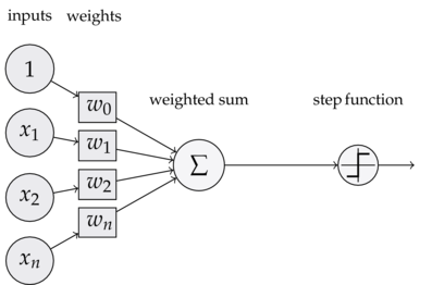
A perceptron classifier is a simple model of a neuron. It has different inputs
($x_1$…$x_n$) with different weights ($w_1$…$w_n$).
The weighted sum $s$ of these inputs is then passed through a step function $f$
(usually a Heaviside step function).
To make things cleaner, here’s a little diagram:
Python!
Here’s a simple version of such a perceptron using Python and NumPy. It will
take two inputs and learn to act like the logical OR function. First, let’s
import some libraries we need:
from random import choice
from numpy import array, dot, random
Then let’s create the step function. In reference to Mathematica, I’ll call
this function unit_step.
unit_step = lambda x: 0 if x < 0 else 1
Next we need to map the possible input to the expected output. The first two
entries of the NumPy array in each tuple are the two input values. The second
element of the tuple is the expected result. And the third entry of the array is
a “dummy” input (also called the bias) which is needed to move the threshold
(also known as the decision boundary) up or down as needed by the step function.
Its value is always 1, so that its influence on the result can be controlled by
its weight.
training_data = [
    (array([0,0,1]), 0),
    (array([0,1,1]), 1),
    (array([1,0,1]), 1),
    (array([1,1,1]), 1),
]
As you can see, this training sequence maps exactly to the definition of the OR
function:
| A | B | A OR B |
|---|---|---|
| 0 | 0 | 0 |
| 0 | 1 | 1 |
| 1 | 0 | 1 |
| 1 | 1 | 1 |
Next we’ll choose three random numbers between 0 and 1 as the initial weights:
w = random.rand(3)
Now on to some variable initializations. The errors list is only used to
store the error values so that they can be plotted later on. If you don’t want
to do any plotting, you can just leave it away. The eta variable controls
the learning rate. And n specifies the number of learning iterations.
errors = []
eta = 0.2
n = 100
In order to find the ideal values for the weights w, we try to reduce the
error magnitude to zero. In this simple case n = 100 iterations are enough;
for a bigger and possibly “noisier” set of input data much larger numbers should
be used.
First we get a random input set from the training data. Then we calculate the
dot product (sometimes also called scalar product or inner product) of the input
and weight vectors. This is our (scalar) result, which we can compare to the
expected value. If the expected value is bigger, we need to increase the
weights, if it’s smaller, we need to decrease them. This correction factor is
calculated in the last line, where the error is multiplied with the learning
rate (eta) and the input vector (x). It is then added to the weights
vector, in order to improve the results in the next iteration.
for i in xrange(n):
    x, expected = choice(training_data)
    result = dot(w, x)
    error = expected - unit_step(result)
    errors.append(error)
    w += eta * error * x
And that’s already everything we need in order to train the perceptron! It has
now “learned” to act like a logical OR function:
for x, _ in training_data:
    result = dot(x, w)
    print("{}: {} -> {}".format(x[:2], result, unit_step(result)))

[0 0]: -0.0714566687173 -> 0
[0 1]: 0.829739696273 -> 1
[1 0]: 0.345454042997 -> 1
[1 1]: 1.24665040799 -> 1
If you’re interested, you can also plot the errors, which is a great way to
visualize the learning process:
from pylab import plot, ylim
ylim([-1,1])
plot(errors)
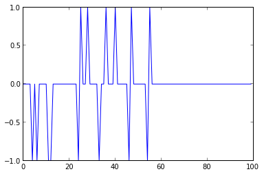
It’s easy to see that the errors stabilize around the 60th iteration. If you
doubt that the errors are definitely eliminated, you can re-run the training
with an iteration count of 500 or more and plot the errors:
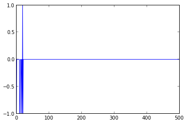
You could also try to change the training sequence in order to model an AND, NOR
or NOT function. Note that it’s not possible to model an XOR function using a
single perceptron like this, because the two classes (0 and 1) of an XOR
function are not linearly separable. In that case you would have to use multiple
layers of perceptrons (which is basically a small neural network).
Wrap Up
Here’s the entire code:
from random import choice
from numpy import array, dot, random

unit_step = lambda x: 0 if x < 0 else 1

training_data = [
    (array([0,0,1]), 0),
    (array([0,1,1]), 1),
    (array([1,0,1]), 1),
    (array([1,1,1]), 1),
]

w = random.rand(3)
errors = []
eta = 0.2
n = 100

for i in xrange(n):
    x, expected = choice(training_data)
    result = dot(w, x)
    error = expected - unit_step(result)
    errors.append(error)
    w += eta * error * x

for x, _ in training_data:
    result = dot(x, w)
    print("{}: {} -> {}".format(x[:2], result, unit_step(result)))
If you have any questions, or if you’ve discovered an error (which is easily
possible as I’ve just learned about this stuff), feel free to leave a comment
below.