Machine Learning Walkthrough Part One: Preparing the Data

Cleaning and preparing data is a critical first step in any machine learning project. In this blog post, Dataquest student Daniel Osei’s takes us through examining a dataset, selecting columns for features, exploring the data visually and then encoding the features for machine learning.

This post is based on a Dataquest ‘Monthly Challenge’, where our students are given a free-form task to complete.

After first reading about Machine Learning on Quora in 2015, Daniel became excited at the prospect of an area that could combine his love of Mathematics and Programming. After reading this article on how to learn data science, Daniel started following the steps, eventually joining Dataquest to learn Data Science with us in in April 2016.

We’d like to thank Daniel for his hard work, and generously letting us publish this post. This walkthrough uses Python 3.5 and Jupyter notebook.

Machine Learning Challenge Overview

Lending Club is a marketplace for personal loans that matches borrowers who are seeking a loan with investors looking to lend money and make a return. Each borrower fills out a comprehensive application, providing their past financial history, the reason for the loan, and more. Lending Club evaluates each borrower’s credit score using past historical data (and their own data science process!) and assigns an interest rate to the borrower.

The Lending Club website.

The loan is then listed on the Lending Club marketplace. You can read more about their marketplace here.

Investors are primarily interested in receiving a return on their investments. Approved loans are listed on the Lending Club website, where qualified investors can browse recently approved loans, the borrower’s credit score, the purpose for the loan, and other information from the application.

Once an investor decides to fund a loan, the borrower then makes monthly payments back to Lending Club. Lending Club redistributes these payments to the investors. This means that investors don’t have to wait until the full amount is paid off to start to see money back. If a loan is fully paid off on time, the investors make a return which corresponds to the interest rate the borrower had to pay in addition to the requested amount. Many loans aren’t completely paid off on time, however, and some borrowers default on the loan.

The Challenge

Suppose an investor has approached us and has asked us to build a machine learning model that can reliably predict if a loan will be paid off or not. This investor described himself/herself as a conservative investor who only wants to invest in loans that have a good chance of being paid off on time. Thus, this client is more interested in a machine learning model which does a good job of filtering out high percentage of loan defaulters.

Our task is to construct a machine learning model that achieves a True Positive Rate of greater than 70% while maintaining a False Positive Rate of less than 7%.

1. Examining the Data Set

Lending Club periodically releases data for all the approved and declined loan applications on their website. You can select different year ranges to download the dataset (in CSV format) for both approved and declined loans.

You’ll also find a data dictionary (in XLS format), towards the bottom of the page, which contains information on the different column names. The data dictionary is useful to help understand what a column represents in the dataset.

The data dictionary contains two sheets:

• LoanStats sheet: describes the approved loans dataset
• RejectStats sheet: describes the rejected loans dataset

We’ll be using the LoanStats sheet since we’re interested in the approved loans dataset.

The approved loans dataset contains information on current loans, completed loans, and defaulted loans. For this challenge, we’ll be working with approved loans data for the years 2007 to 2011.

First, lets import some of the libraries that we’ll be using, and set some parameters to make the output easier to read.

import pandas as pd
import numpy as np
pd.set_option('max_columns', 120)
pd.set_option('max_colwidth', 5000)


import matplotlib.pyplot as plt
import seaborn as sns
%matplotlib inline
plt.rcParams['figure.figsize'] = (12,8)

Loading The Data Into Pandas DataFrame

We’ve downloaded our dataset and named it lending_club_loans.csv, but now we need to load it into a pandas DataFrame to explore it.

To ensure that code run fast for us, we need to reduce the size of lending_club_loans.csv by doing the following:

• Remove the first line: It contains extraneous text instead of the column titles. This text prevents the dataset from being parsed properly by the pandas library.
• Remove the ‘desc’ column: it contains a long text explanation for the loan.
• Remove the ‘url’ column: it contains a link to each on Lending Club which can only be accessed with an investor account.
• Removing all columns with more than 50% missing values: This allows us to move faster since don’t need to spend time trying to fill these values.

We’ll also name the filtered dataset loans_2007 and later at the end of this section save it as loans_2007.csv to keep it separate from the raw data. This is good practice and makes sure we have our original data in case we need to go back and retrieve any of the original data we’re removing.

Now, let’s go ahead and perform these steps:

# skip row 1 so pandas can parse the data properly.
loans_2007 = pd.read_csv('data/lending_club_loans.csv', skiprows=1, low_memory=False) 
half_count = len(loans_2007) / 2
loans_2007 = loans_2007.dropna(thresh=half_count,axis=1) # Drop any column with more than 50% missing values
loans_2007 = loans_2007.drop(['url','desc'],axis=1)      # These columns are not useful for our purposes

Let’s use the pandas head() method to display first three rows of the loans_2007 DataFrame, just to make sure we were able to load the dataset properly:

loans_2007.head(3)

Let’s also use pandas .shape attribute to view the number of samples and features we’re dealing with at this stage:

loans_2007.shape

(42538, 56)

2. Narrowing down our columns

It’s a great idea to spend some time to familiarize ourselves with the columns in the dataset, to understand what each feature represents. This is important, because a poor understanding of the features could cause us to make mistakes in the data analysis and the modeling process.

We’ll be using the data dictionary Lending Club provided to help us become familiar with the columns and what each represents in the dataset. To make the process easier, we’ll create a DataFrame to contain the names of the columns, data type, first row’s values, and description from the data dictionary.

To make this easier, we’ve pre-converted the data dictionary from Excel format to a CSV.

data_dictionary = pd.read_csv('LCDataDictionary.csv') # Loading in the data dictionary
print(data_dictionary.shape[0])
print(data_dictionary.columns.tolist())

117
['LoanStatNew', 'Description']

data_dictionary.head()
data_dictionary = data_dictionary.rename(columns={'LoanStatNew': 'name',
                                                 'Description': 'description'})

Now that we’ve got the data dictionary loaded, let’s join the first row of loans_2007 to the data_dictionary DataFrame to give us a preview DataFrame with the following columns:

• name – contains the column names of loans_2007.
• dtypes – contains the data types of the loans_2007 columns.
• first value – contains the values of loans_2007 first row.
• description – explains what each column in loans_2007 represents.

loans_2007_dtypes = pd.DataFrame(loans_2007.dtypes,columns=['dtypes'])
loans_2007_dtypes = loans_2007_dtypes.reset_index()
loans_2007_dtypes['name'] = loans_2007_dtypes['index']
loans_2007_dtypes = loans_2007_dtypes[['name','dtypes']]

loans_2007_dtypes['first value'] = loans_2007.loc[0].values
preview = loans_2007_dtypes.merge(data_dictionary, on='name',how='left')

preview.head()

When we printed the shape of loans_2007 earlier, we noticed that it had 56 columns which also means this preview DataFrame has 56 rows. It can be cumbersome to try to explore all the rows of preview at once, so instead we’ll break it up into three parts and look at smaller selection of features each time.

As you explore the features to better understand each of them, you’ll want to pay attention to any column that:

• leaks information from the future (after the loan has already been funded),
• don’t affect the borrower’s ability to pay back the loan (e.g. a randomly generated ID value by Lending Club),
• is formatted poorly,
• requires more data or a lot of preprocessing to turn into useful a feature, or
• contains redundant information.

I’ll say it again to emphasize it because it’s important: We need to especially pay close attention to data leakage, which can cause the model to overfit. This is because the model would be also learning from features that wouldn’t be available when we’re using it make predictions on future loans.

First Group Of Columns

Let’s display the first 19 rows of preview and analyze them:

preview[:19]

After analyzing the columns, we can conclude that the following features can be removed:

• id – randomly generated field by Lending Club for unique identification purposes only.
• member_id – also randomly generated field by Lending Club for identification purposes only.
• funded_amnt – leaks information from the future(after the loan is already started to be funded).
• funded_amnt_inv – also leaks data from the future.
• sub_grade – contains redundant information that is already in the grade column (more below).
• int_rate – also included within the grade column.
• emp_title – requires other data and a lot of processing to become potentially useful
• issued_d – leaks data from the future.

Lending Club uses a borrower’s grade and payment term (30 or months) to assign an interest rate (you can read more about Rates & Fees). This causes variations in interest rate within a given grade. But, what may be useful for our model is to focus on clusters of borrowers instead of individuals. And, that’s exactly what grading does – it segments borrowers based on their credit score and other behaviors, which is we should keep the grade column and drop interest int_rate and sub_grade.

Let’s drop these columns from the DataFrame before moving onto to the next group of columns.

drop_list = ['id','member_id','funded_amnt','funded_amnt_inv',
             'int_rate','sub_grade','emp_title','issue_d']
loans_2007 = loans_2007.drop(drop_list,axis=1)

Second Group Of Columns

Let’s move on to the next 19 columns:

preview[19:38]

In this group,take note of the fico_range_low and fico_range_high columns. Both are in this second group of columns but because they related to some other columns, we’ll talk more about them after looking at the last group of columns.

We can drop the following columns:

• zip_code – mostly redundant with the addr_state column since only the first 3 digits of the 5 digit zip code are visible.
• out_prncp – leaks data from the future.
• out_prncp_inv – also leaks data from the future.
• total_pymnt – also leaks data from the future.
• total_pymnt_inv – also leaks data from the future.

Let’s go ahead and remove these 5 columns from the DataFrame:

drop_cols = [ 'zip_code','out_prncp','out_prncp_inv',
             'total_pymnt','total_pymnt_inv']
loans_2007 = loans_2007.drop(drop_cols, axis=1)

Third Group Of Columns

Let’s analyze the last group of features:

preview[38:]

In this last group of columns, we need to drop the following, all of which leak data from the future:

• total_rec_prncp
• total_rec_int
• total_rec_late_fee
• recoveries
• collection_recovery_fee
• last_pymnt_d
• last_pymnt_amnt

Let’s drop our last group of columns:

drop_cols = ['total_rec_prncp','total_rec_int', 'total_rec_late_fee',
             'recoveries', 'collection_recovery_fee', 'last_pymnt_d',
             'last_pymnt_amnt']

loans_2007 = loans_2007.drop(drop_cols, axis=1)

Investigating FICO Score Columns

Now, besides the explanations provided here in the Description column,let’s learn more about fico_range_low, fico_range_high, last_fico_range_low, and last_fico_range_high.

FICO scores are a credit score, or a number used by banks and credit cards to represent how credit-worthy a person is. While there are a few types of credit scores used in the United States, the FICO score is the best known and most widely used.

When a borrower applies for a loan, Lending Club gets the borrowers credit score from FICO – they are given a lower and upper limit of the range that the borrowers score belongs to, and they store those values as fico_range_low, fico_range_high. After that, any updates to the borrowers score are recorded as last_fico_range_low, and last_fico_range_high.

A key part of any data science project is to do everything you can to understand the data. While researching this data set, I found a project done in 2014 by a group of students from Stanford University on this same dataset.

In the report for the project, the group listed the current credit score (last_fico_range) among late fees and recovery fees as fields they mistakenly added to the features but state that they later learned these columns all leak information into the future.

However, following this group’s project, another group from Stanford worked on this same Lending Club dataset. They used the FICO score columns, dropping only last_fico_range_low, in their modeling. This second group’s report described last_fico_range_high as the one of the more important features in predicting accurate results.

The question we must answer is, do the FICO credit scores information into the future? Recall a column is considered leaking information when especially it won’t be available at the time we use our model – in this case when we use our model on future loans.

This blog examines in-depth the FICO scores for lending club loans, and notes that while looking at the trend of the FICO scores is a great predictor of whether a loan will default, that because FICO scores continue to be updated by the Lending Club after a loan is funded, a defaulting loan can lower the borrowers score, or in other words, will leak data.

Therefore we can safely use fico_range_low and fico_range_high, but not last_fico_range_low, and last_fico_range_high. Lets take a look at the values in these columns:

print(loans_2007['fico_range_low'].unique())
print(loans_2007['fico_range_high'].unique())

[ 735.  740.  690.  695.  730.  660.  675.  725.  710.  705.  720.  665.
  670.  760.  685.  755.  680.  700.  790.  750.  715.  765.  745.  770.
  780.  775.  795.  810.  800.  815.  785.  805.  825.  820.  630.  625.
   nan  650.  655.  645.  640.  635.  610.  620.  615.]
[ 739.  744.  694.  699.  734.  664.  679.  729.  714.  709.  724.  669.
  674.  764.  689.  759.  684.  704.  794.  754.  719.  769.  749.  774.
  784.  779.  799.  814.  804.  819.  789.  809.  829.  824.  634.  629.
   nan  654.  659.  649.  644.  639.  614.  624.  619.]

Let’s get rid of the missing values, then plot histograms to look at the ranges of the two columns:

fico_columns = ['fico_range_high','fico_range_low']

print(loans_2007.shape[0])
loans_2007.dropna(subset=fico_columns,inplace=True)
print(loans_2007.shape[0])

loans_2007[fico_columns].plot.hist(alpha=0.5,bins=20);

42538
42535

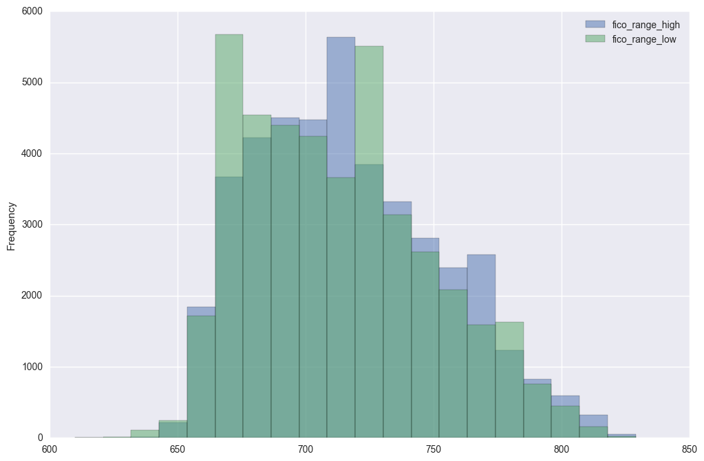
Let’s now go ahead and create a column for the average of fico_range_low and fico_range_high columns and name it fico_average. Note that this is not the average FICO score for each borrower, but rather an average of the high and low range that we know the borrower is in.

loans_2007['fico_average'] = (loans_2007['fico_range_high'] + loans_2007['fico_range_low']) / 2

Let’s check what we just did.

cols = ['fico_range_low','fico_range_high','fico_average']
loans_2007[cols].head()

Good! We got the mean calculations and everything right. Now, we can go ahead and drop fico_range_low, fico_range_high, last_fico_range_low, and last_fico_range_high columns.

drop_cols = ['fico_range_low','fico_range_high','last_fico_range_low',
             'last_fico_range_high']
loans_2007 = loans_2007.drop(drop_cols, axis=1)
loans_2007.shape

(42535, 33)

Notice just by becoming familiar with the columns in the dataset, we’re able to reduce the number of columns from 56 to 33.

Decide On A Target Column

Now, let’s decide on the appropriate column to use as a target column for modeling – keep in mind the main goal is predict who will pay off a loan and who will default.

We learned from the description of columns in the preview DataFrame that loan_status is the only field in the main dataset that describe a loan status, so let’s use this column as the target column.

preview[preview.name == 'loan_status']

Currently, this column contains text values that need to be converted to numerical values to be able use for training a model.

Let’s explore the different values in this column and come up with a strategy for converting the values in this column. We’ll use the DataFrame method value_counts() to return the frequency of the unique values in the loan_status column.

loans_2007["loan_status"].value_counts()

Fully Paid                                             33586
Charged Off                                             5653
Does not meet the credit policy. Status:Fully Paid      1988
Does not meet the credit policy. Status:Charged Off      761
Current                                                  513
In Grace Period                                           16
Late (31-120 days)                                        12
Late (16-30 days)                                          5
Default                                                    1
Name: loan_status, dtype: int64

The loan status has nine different possible values!

Let’s learn about these unique values to determine the ones that best describe the final outcome of a loan, and also the kind of classification problem we’ll be dealing with.

You can read about most of the different loan statuses on the Lending Club website as well as these posts on the Lend Academy and Orchard forums. I have pulled that data together in a table below so we can see the unique values, their frequency in the dataset and what each means:

meaning = [
    "Loan has been fully paid off.",
    "Loan for which there is no longer a reasonable expectation of further payments.",
    "While the loan was paid off, the loan application today would no longer meet the credit policy and wouldn't be approved on to the marketplace.",
    "While the loan was charged off, the loan application today would no longer meet the credit policy and wouldn't be approved on to the marketplace.",
    "Loan is up to date on current payments.",
    "The loan is past due but still in the grace period of 15 days.",
    "Loan hasn't been paid in 31 to 120 days (late on the current payment).",
    "Loan hasn't been paid in 16 to 30 days (late on the current payment).",
    "Loan is defaulted on and no payment has been made for more than 121 days."]

status, count = loans_2007["loan_status"].value_counts().index, loans_2007["loan_status"].value_counts().values

loan_statuses_explanation = pd.DataFrame({'Loan Status': status,'Count': count,'Meaning': meaning})[['Loan Status','Count','Meaning']]
loan_statuses_explanation

Remember, our goal is to build a machine learning model that can learn from past loans in trying to predict which loans will be paid off and which won’t. From the above table, only the Fully Paid and Charged Off values describe the final outcome of a loan. The other values describe loans that are still on going, and even though some loans are late on payments, we can’t jump the gun and classify them as Charged Off.

Also, while the Default status resembles the Charged Off status, in Lending Club’s eyes, loans that are charged off have essentially no chance of being repaid while default ones have a small chance. Therefore, we should use only samples where the loan_status column is 'Fully Paid' or 'Charged Off'.

We’re not interested in any statuses that indicate that the loan is ongoing or in progress, because predicting that something is in progress doesn’t tell us anything.

Since we’re interested in being able to predict which of these 2 values a loan will fall under, we can treat the problem as binary classification.

Let’s remove all the loans that don’t contain either 'Fully Paid' or 'Charged Off' as the loan’s status and then transform the 'Fully Paid' values to 1 for the positive case and the 'Charged Off' values to 0 for the negative case.

This will mean that out of the ~42,000 rows we have, we’ll be removing just over 3,000.

There are few different ways to transform all of the values in a column, we’ll use the DataFrame method replace().

loans_2007 = loans_2007[(loans_2007["loan_status"] == "Fully Paid") |
                            (loans_2007["loan_status"] == "Charged Off")]

mapping_dictionary = {"loan_status":{ "Fully Paid": 1, "Charged Off": 0}}
loans_2007 = loans_2007.replace(mapping_dictionary)

Visualizing the Target Column Outcomes

fig, axs = plt.subplots(1,2,figsize=(14,7))
sns.countplot(x='loan_status',data=filtered_loans,ax=axs[0])
axs[0].set_title("Frequency of each Loan Status")
filtered_loans.loan_status.value_counts().plot(x=None,y=None, kind='pie', ax=axs[1],autopct='%1.2f%%')
axs[1].set_title("Percentage of each Loan status")
plt.show()

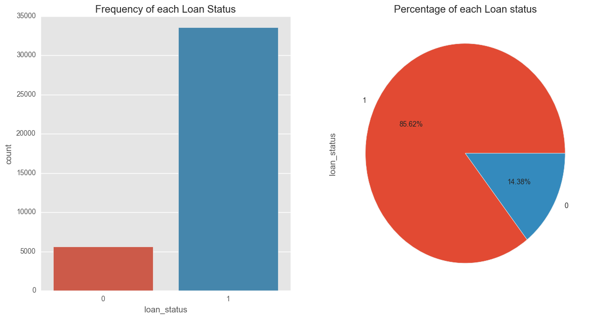
These plots indicate that a significant number of borrowers in our dataset paid off their loan – 85.62% of loan borrowers paid off amount borrowed, while 14.38% unfortunately defaulted. From our loan data it is these ‘defaulters’ that we’re more interested in filtering out as much as possible to reduce loses on investment returns.

In part two of our walkthrough, we’ll learn that the significant percentage difference, or class imbalance, in target variable needs to be considered when we build our model.

Remove Columns with only One Value

To wrap up this section, let’s look for any columns that contain only one unique value and remove them. These columns won’t be useful for the model since they don’t add any information to each loan application. In addition, removing these columns will reduce the number of columns we’ll need to explore further in the next stage.

The pandas Series method nunique() returns the number of unique values, excluding any null values. We can use apply this method across the dataset to remove these columns in one easy step.

loans_2007 = loans_2007.loc[:,loans_2007.apply(pd.Series.nunique) != 1]

Again, there may be some columns with more than one unique values but one of the values has insignificant frequency in the dataset. Let’s find out and drop such column(s):

for col in loans_2007.columns:
    if (len(loans_2007[col].unique()) < 4):
        print(loans_2007[col].value_counts())
        print()

 36 months    29096
 60 months    10143
Name: term, dtype: int64

Not Verified       16845
Verified           12526
Source Verified     9868
Name: verification_status, dtype: int64

1    33586
0     5653
Name: loan_status, dtype: int64

n    39238
y        1
Name: pymnt_plan, dtype: int64

The payment plan column (pymnt_plan) has two unique values, 'y' and 'n', with 'y' occurring only once. Let’s drop this column:

print(loans_2007.shape[1])
loans_2007 = loans_2007.drop('pymnt_plan', axis=1)
print("We've been able to reduced the features to => {}".format(loans_2007.shape[1]))

25
We've been able to reduced the features to => 24

Lastly, lets save our work in this section to a CSV file.

loans_2007.to_csv("processed_data/filtered_loans_2007.csv",index=False)

3. Preparing the Features for Machine Learning

In this section, we’ll prepare the filtered_loans_2007.csv data for machine learning. We’ll focus on handling missing values, converting categorical columns to numeric columns and removing any other extraneous columns.

We need to handle missing values and categorical features before feeding the data into a machine learning algorithm, because the mathematics underlying most machine learning models assumes that the data is numerical and contains no missing values. To reinforce this requirement, scikit-learn will return an error if you try to train a model using data that contain missing values or non-numeric values when working with models like linear regression and logistic regression.

Here’s an outline of what we’ll be doing in this stage:

• Handle Missing Values
• Investigate Categorical Columns
  • Convert Categorical Columns To Numeric Features
    • Map Ordinal Values To Integers
    • Encode Nominal Values As Dummy Variables

First though, let’s load in the data from last section’s final output:

filtered_loans = pd.read_csv('processed_data/filtered_loans_2007.csv')
print(filtered_loans.shape)
filtered_loans.head()

(39239, 24)

Handle Missing Values

Let’s compute the number of missing values and determine how to handle them. We can return the number of missing values across the DataFrame by:

• First, use the Pandas DataFrame method isnull() to return a DataFrame containing Boolean values:
  • True if the original value is null
  • False if the original value isn’t null
• Then, use the Pandas DataFrame method sum() to calculate the number of null values in each column.

null_counts = filtered_loans.isnull().sum()
print("Number of null values in each column:n{}".format(null_counts))

Number of null values in each column:
loan_amnt                 0
term                      0
installment               0
grade                     0
emp_length                0
home_ownership            0
annual_inc                0
verification_status       0
loan_status               0
purpose                   0
title                    10
addr_state                0
dti                       0
delinq_2yrs               0
earliest_cr_line          0
inq_last_6mths            0
open_acc                  0
pub_rec                   0
revol_bal                 0
revol_util               50
total_acc                 0
last_credit_pull_d        2
pub_rec_bankruptcies    697
fico_average              0
dtype: int64

Notice while most of the columns have 0 missing values, title has 9 missing values, revol_util has 48, and pub_rec_bankruptcies contains 675 rows with missing values. Let’s remove columns entirely where more than 1% (392) of the rows for that column contain a null value. In addition, we’ll remove the remaining rows containing null values, which means we’ll lose a bit of data, but in return keep some extra features to use for prediction.

This means that we’ll keep the title and revol_util columns, just removing rows containing missing values, but drop the pub_rec_bankruptcies column entirely since more than 1% of the rows have a missing value for this column.

Here’s a list of steps we can use to achieve that:

• Use the drop method to remove the pub_rec_bankruptcies column from filtered_loans.
• Use the dropna method to remove all rows from filtered_loans containing any missing values.

filtered_loans = filtered_loans.drop("pub_rec_bankruptcies",axis=1)
filtered_loans = filtered_loans.dropna()

Next, we’ll focus on the categorical columns.

Investigate Categorical Columns

Keep in mind, the goal in this section is to have all the columns as numeric columns (int or float data type), and containing no missing values. We just dealt with the missing values, so let’s now find out the number of columns that are of the object data type and then move on to process them into numeric form.

print("Data types and their frequencyn{}".format(filtered_loans.dtypes.value_counts()))

Data types and their frequency
float64    11
object     11
int64       1
dtype: int64

We have 11 object columns that contain text which need to be converted into numeric features. Let’s select just the object columns using the DataFrame method select_dtype, then display a sample row to get a better sense of how the values in each column are formatted.

object_columns_df = filtered_loans.select_dtypes(include=['object'])
print(object_columns_df.iloc[0])

term                     36 months
grade                            B
emp_length               10+ years
home_ownership                RENT
verification_status       Verified
purpose                credit_card
title                     Computer
addr_state                      AZ
earliest_cr_line          Jan-1985
revol_util                   83.7%
last_credit_pull_d        Sep-2016
Name: 0, dtype: object

Notice that revol_util column contains numeric values, but is formatted as object. We learned from the description of columns in the preview DataFrame earlier that revol_util is a revolving line utilization rate or the amount of credit the borrower is using relative to all available credit (read more here).

We need to format revol_util as numeric values. Here’s what we should do:

• Use the str.rstrip() string method to strip the right trailing percent sign (%).
• On the resulting Series object, use the astype() method to convert to the type float.
• Assign the new Series of float values back to the revol_util column in the filtered_loans.

filtered_loans['revol_util'] = filtered_loans['revol_util'].str.rstrip('%').astype('float')

Moving on, these columns seem to represent categorical values:

• home_ownership – home ownership status, can only be 1 of 4 categorical values according to the data dictionary.
• verification_status – indicates if income was verified by Lending Club.
• emp_length – number of years the borrower was employed upon time of application.
• term – number of payments on the loan, either 36 or 60.
• addr_state – borrower’s state of residence.
• grade – LC assigned loan grade based on credit score.
• purpose – a category provided by the borrower for the loan request.
• title – loan title provided the borrower.

To be sure, lets confirm by checking the number of unique values in each of them.

Also, based on the first row’s values for purpose and title, it appears these two columns reflect the same information. We’ll explore their unique value counts separately to confirm if this is true.

Lastly, notice the first row’s values for both earliest_cr_line and last_credit_pull_d columns contain date values that would require a good amount of feature engineering for them to be potentially useful:

• earliest_cr_line – The month the borrower’s earliest reported credit line was opened
• last_credit_pull_d – The most recent month Lending Club pulled credit for this loan

We’ll remove these date columns from the DataFrame.

First, let’s explore the unique value counts of the six columns that seem like they contain categorical values

cols = ['home_ownership', 'grade','verification_status', 'emp_length', 'term', 'addr_state']
for name in cols:
    print(name,':')
    print(object_columns_df[name].value_counts(),'n')

home_ownership :
RENT        18677
MORTGAGE    17381
OWN          3020
OTHER          96
NONE            3
Name: home_ownership, dtype: int64 

grade :
B    11873
A    10062
C     7970
D     5194
E     2760
F     1009
G      309
Name: grade, dtype: int64 

verification_status :
Not Verified       16809
Verified           12515
Source Verified     9853
Name: verification_status, dtype: int64 

emp_length :
10+ years    8715
< 1 year     4542
2 years      4344
3 years      4050
4 years      3385
5 years      3243
1 year       3207
6 years      2198
7 years      1738
8 years      1457
9 years      1245
n/a          1053
Name: emp_length, dtype: int64 

term :
 36 months    29041
 60 months    10136
Name: term, dtype: int64 

addr_state :
CA    7019
NY    3757
FL    2831
TX    2693
NJ    1825
IL    1513
PA    1493
VA    1388
GA    1381
MA    1322
OH    1197
MD    1039
AZ     863
WA     830
CO     777
NC     772
CT     738
MI     718
MO     677
MN     608
NV     488
SC     469
WI     447
OR     441
AL     441
LA     432
KY     319
OK     294
KS     264
UT     255
AR     241
DC     211
RI     197
NM     187
WV     174
HI     170
NH     169
DE     113
MT      84
WY      83
AK      79
SD      61
VT      53
MS      19
TN      17
IN       9
ID       6
IA       5
NE       5
ME       3
Name: addr_state, dtype: int64 

Most of these coumns contain discrete categorical values which we can encode as dummy variables and keep. The addr_state column, however,contains too many unique values, so it’s better to drop this.

Next, let’s look at the unique value counts for the purpose and title columns to understand which columns we want to keep.

for name in ['purpose','title']:
    print("Unique Values in column: {}n".format(name))
    print(filtered_loans[name].value_counts(),'n')

Unique Values in column: purpose

debt_consolidation    18355
credit_card            5073
other                  3921
home_improvement       2944
major_purchase         2178
small_business         1792
car                    1534
wedding                 940
medical                 688
moving                  580
vacation                377
house                   372
educational             320
renewable_energy        103
Name: purpose, dtype: int64 

Unique Values in column: title

Debt Consolidation                         2142
Debt Consolidation Loan                    1670
Personal Loan                               650
Consolidation                               501
debt consolidation                          495
Credit Card Consolidation                   354
Home Improvement                            350
Debt consolidation                          331
Small Business Loan                         317
Credit Card Loan                            310
Personal                                    306
Consolidation Loan                          255
Home Improvement Loan                       243
personal loan                               231
personal                                    217
Loan                                        210
Wedding Loan                                206
Car Loan                                    198
consolidation                               197
Other Loan                                  187
Credit Card Payoff                          153
Wedding                                     152
Major Purchase Loan                         144
Credit Card Refinance                       143
Consolidate                                 126
Medical                                     120
Credit Card                                 115
home improvement                            109
My Loan                                      94
Credit Cards                                 92
                                           ... 
toddandkim4ever                               1
Remainder of down payment                     1
Building a Financial Future                   1
Higher interest payoff                        1
Chase Home Improvement Loan                   1
Sprinter Purchase                             1
Refi credit card-great payment record         1
Karen's Freedom Loan                          1
Business relocation and partner buyout        1
Update My New House                           1
tito                                          1
florida vacation                              1
Back to 0                                     1
Bye Bye credit card                           1
britschool                                    1
Consolidation 16X60                           1
Last Call                                     1
Want to be debt free in "3"                   1
for excellent credit                          1
loaney                                        1
jamal's loan                                  1
Refying Lending Club-I LOVE THIS PLACE!       1
Consoliation Loan                             1
Personal/ Consolidation                       1
Pauls Car                                     1
Road to freedom loan                          1
Pay it off FINALLY!                           1
MASH consolidation                            1
Destination Wedding                           1
Store Charge Card                             1
Name: title, dtype: int64 

It appears the purpose and title columns do contain overlapping information, but the purpose column contains fewer discrete values and is cleaner, so we’ll keep it and drop title.

Lets drop the columns we’ve decided not to keep so far:

drop_cols = ['last_credit_pull_d','addr_state','title','earliest_cr_line']
filtered_loans = filtered_loans.drop(drop_cols,axis=1)

Convert Categorical Columns to Numeric Features

First, let’s understand the two types of categorical features we have in our dataset and how we can convert each to numerical features:

• Ordinal values: these categorical values are in natural order. That’s you can sort or order them either in increasing or decreasing order. For instance, we learnt earlier that Lending Club grade loan applicants from A to G, and assign each applicant a corresponding interest rate – grade A is less riskier while grade B is riskier than A in that order:

A < B < C < D < E < F < G ; where < means less riskier than

• Nominal Values: these are regular categorical values. You can’t order nominal values. For instance, while we can order loan applicants in the employment length column (emp_length) based on years spent in the workforce:

year 1 < year 2 < year 3 … < year N,

we can’t do that with the column purpose. It wouldn’t make sense to say:

car < wedding < education < moving < house

These are the columns we now have in our dataset:

• Ordinal Values
  • grade
  • emp_length
• Nominal Values _ home_ownership
  • verification_status
  • purpose
  • term

There are different approaches to handle each of these two types. In the steps following, we’ll convert each of them accordingly.

To map the ordinal values to integers, we can use the pandas DataFrame method replace() to map both grade and emp_length to appropriate numeric values

mapping_dict = {
    "emp_length": {
        "10+ years": 10,
        "9 years": 9,
        "8 years": 8,
        "7 years": 7,
        "6 years": 6,
        "5 years": 5,
        "4 years": 4,
        "3 years": 3,
        "2 years": 2,
        "1 year": 1,
        "< 1 year": 0,
        "n/a": 0
 
    },
    "grade":{
        "A": 1,
        "B": 2,
        "C": 3,
        "D": 4,
        "E": 5,
        "F": 6,
        "G": 7
    }
}

filtered_loans = filtered_loans.replace(mapping_dict)
filtered_loans[['emp_length','grade']].head()

Perfect! Let’s move on to the Nominal Values. The approach to converting nominal features into numerical features is to encode them as dummy variables. The process will be:

• Use pandas’ get_dummies() method to return a new DataFrame containing a new column for each dummy variable
• Use the concat() method to add these dummy columns back to the original DataFrame
• Then drop the original columns entirely using the drop method

Lets’ go ahead and encode the nominal columns that we now have in our dataset.

nominal_columns = ["home_ownership", "verification_status", "purpose", "term"]
dummy_df = pd.get_dummies(filtered_loans[nominal_columns])
filtered_loans = pd.concat([filtered_loans, dummy_df], axis=1)
filtered_loans = filtered_loans.drop(nominal_columns, axis=1)

filtered_loans.head()

To wrap things up, let’s inspect our final output from this section to make sure all the features are of the same length, contain no null value, and are numericals.

Let’s use pandas info method to inspect the filtered_loans DataFrame:

filtered_loans.info()

<class 'pandas.core.frame.DataFrame'>
Int64Index: 39177 entries, 0 to 39238
Data columns (total 39 columns):
loan_amnt                              39177 non-null float64
installment                            39177 non-null float64
grade                                  39177 non-null int64
emp_length                             39177 non-null int64
annual_inc                             39177 non-null float64
loan_status                            39177 non-null int64
dti                                    39177 non-null float64
delinq_2yrs                            39177 non-null float64
inq_last_6mths                         39177 non-null float64
open_acc                               39177 non-null float64
pub_rec                                39177 non-null float64
revol_bal                              39177 non-null float64
revol_util                             39177 non-null float64
total_acc                              39177 non-null float64
fico_average                           39177 non-null float64
home_ownership_MORTGAGE                39177 non-null uint8
home_ownership_NONE                    39177 non-null uint8
home_ownership_OTHER                   39177 non-null uint8
home_ownership_OWN                     39177 non-null uint8
home_ownership_RENT                    39177 non-null uint8
verification_status_Not Verified       39177 non-null uint8
verification_status_Source Verified    39177 non-null uint8
verification_status_Verified           39177 non-null uint8
purpose_car                            39177 non-null uint8
purpose_credit_card                    39177 non-null uint8
purpose_debt_consolidation             39177 non-null uint8
purpose_educational                    39177 non-null uint8
purpose_home_improvement               39177 non-null uint8
purpose_house                          39177 non-null uint8
purpose_major_purchase                 39177 non-null uint8
purpose_medical                        39177 non-null uint8
purpose_moving                         39177 non-null uint8
purpose_other                          39177 non-null uint8
purpose_renewable_energy               39177 non-null uint8
purpose_small_business                 39177 non-null uint8
purpose_vacation                       39177 non-null uint8
purpose_wedding                        39177 non-null uint8
term_ 36 months                        39177 non-null uint8
term_ 60 months                        39177 non-null uint8
dtypes: float64(12), int64(3), uint8(24)
memory usage: 5.7 MB

Save to CSV

It is a good practice to store the final output of each section or stage of your workflow in a separate csv file. One of the benefits of this practice is that it helps us to make changes in our data processing flow without having to recalculate everything.

filtered_loans.to_csv("processed_data/cleaned_loans_2007.csv",index=False)

Next Steps

In this post, we used the Data Dictionary Lending Club provided with the Loans_2007 DataFrame’s first row’s values to become familiar with the columns in the dataset and were able to removed many columns that aren’t useful for modeling. We also selected loan_status as our target column and decided to focus our modeling efforts on binary classification.

Then, we performed the last amount of data preparation necessary to get the features into data types that can be fed into machine learning algorithms. We converted all columns of object data type(Categorical features) to numerical values because those are the only type of values scikit-learn can work with.

Don’t miss part two of this Machine learning walkthrough, where we’ll experiment with different machine learning algorithms to train, evaluate models performance, tune algorithms hyperparameters, and use the best performing model to fit the whole dataset for deployment.

You can subscribe below to be notified when the final part of our machine learning walkthrough is released.