About David: David Asboth is a Data Scientist with a software development background. He’s had many different job titles over the years, with a common theme: he solves human problems with computers and data. This post originally appeared on his blog, davidasboth.com
Introduction
In Part 1, I introduced the concept of Self-Organising Maps (SOMs). Now in Part 2 I want to step through the process of training and using a SOM – both the intuition and the Python code. At the end I’ll also present a couple of real life use cases, not just the toy example we’ll use for implementation.
The first thing we need is a problem to solve!
I’ll use the colour map as the walkthrough example because it lends itself very nicely to visualisation.
Setup
Dataset
Our data will be a collection of random colours, so first we’ll artificially create a dataset of 100. Each colour is a 3D vector representing R, G and B values:
import numpy as np
raw_data = np.random.randint(0, 255, (3, 100))
That’s simply 100 rows of 3D vectors all between the values of 0 and 255.
Objective
Just to be clear, here’s what we’re trying to do. We want to take our 3D colour vectors and map them onto a 2D surface in such a way that similar colours will end up in the same area of the 2D surface.
SOM Parameters
Before training a SOM we need to decide on a few parameters.
SOM Size
First of all, its dimensionality. In theory, a SOM can be any number of dimensions, but for visualisation purposes it is typically 2D and that’s what I’ll be using too.
We also need to decide the number of neurons in the 2D grid. This is one of those decisions in machine learning that might as well be black magic, so we probably need to try a few sizes to get one that feels right.
Remember, this is unsupervised learning, meaning whatever answer the algorithm comes up with will have to be evaluated somewhat subjectively. It’s typical in an unsupervised problem (e.g. k-means clustering) to do multiple runs and see what works.
I’ll go with a 5 by 5 grid. I guess one rule of thumb should be to use fewer neurons than you have data points, otherwise they might not overlap. As we’ll see we actually want them to overlap, because having multiple 3D vectors mapping to the same point in 2D is how we find similarities between our data points.
One important aspect of the SOM is that each of the 2D points on the grid actually represent a multi-dimensional weight vector. Each point on the SOM has a weight vector associated with it that is the same number of dimensions as our input data, in this case 3 to match the 3 dimensions of our colours. We’ll see why this is important when we go through the implementation.
Learning Parameters
Training the SOM is an iterative process – it will get better at its task with every iteration, so we need a cutoff point. Our problem is quite small so 2,000 iterations should suffice but in bigger problems it’s quite possible to need over 10,000.
We also need a learning rate. The learning rate decides by how much we apply changes to our SOM at each iteration.
If it’s too high, we will keep making drastic changes to the SOM and might never settle on a solution.
If it’s too low, we’ll never get anything done as we will only make very small changes.
In practice it is best to start with a larger learning rate and reduce it slowly over time. This is so that the SOM can start by making big changes but then settle into a solution after a while.
Implementation
For the rest of this post I will use 3D to refer to the dimensionality of the input data (which in reality could be any number of dimensions) and 2D as the dimensionality of the SOM (which we decide and could also be any number).
Setup
To setup the SOM we need to start with the following:
- Decide on and initialise the SOM parameters (as above)
- Setup the grid by creating a 5×5 array of random 3D weight vectors
  network_dimensions = np.array([5, 5])
  n_iterations = 2000
  init_learning_rate = 0.01
  # establish size variables based on data
  m = raw_data.shape[0]
  n = raw_data.shape[1]

  # weight matrix (i.e. the SOM) needs to be one m-dimensional vector for each neuron in the SOM
  net = np.random.random((network_dimensions[0], network_dimensions[1], m))

  # initial neighbourhood radius
  init_radius = max(network_dimensions[0], network_dimensions[1]) / 2
  # radius decay parameter
  time_constant = n_iterations / np.log(init_radius)
Those last two parameters relate to the 2D neighbourhood of each neuron in the SOM during training. We’ll return to those in the learning phase. Like the learning rate, the initial 2D radius will encompass most of the SOM and will gradually decrease as the number of iterations increases.
Normalisation
Another detail to discuss at this point is whether or not we normalise our dataset.
First of all, SOMs train faster (and “better”) if all our values are between 0 and 1. This is often true with machine learning problems, and it’s to avoid one of our dimensions “dominating” the others in the learning process. For example, if one of our variable was salary (in the thousands) and another was height (in metres, so rarely over 2.0) then salary will get a higher importance simply because it has much higher values. Normalising to the unit interval will remove this effect.
In our case all 3 dimensions refer to a value between 0 and 255 so we can normalise the entire dataset at once. However, if our variables were on different scales we would have to do this column by column.
I don’t want this code to be entirely tailored to the colour dataset so I’ll leave the normalisation options tied to a few Booleans that are easy to change.
normalise_data = True

# if True, assume all data is on common scale
# if False, normalise to [0 1] range along each column
normalise_by_column = False

# we want to keep a copy of the raw data for later
data = raw_data

# check if data needs to be normalised
if normalise_data:
    if normalise_by_column:
        # normalise along each column
        col_maxes = raw_data.max(axis=0)
        data = raw_data / col_maxes[np.newaxis, :]
    else:
        # normalise entire dataset
        data = raw_data / data.max()
Now we’re ready to start the learning process.
Learning
In broad terms the learning process will be as follows. We’ll fill in the implementation details as we go along.
For a single iteration:
- Find the neuron in the SOM whose associated 3D vector is closest to our chosen 3D colour vector. At each step, this is called the Best Matching Unit (BMU)
- Move the BMU’s 3D weight vector closer to the input vector in 3D space
- Identify the 2D neighbours of the BMU and also move their 3D weight vectors closer to the input vector, although by a smaller amount
- Update the learning rate (reduce it at each iteration)
And that’s it. By doing the penultimate step, moving the BMU’s neighbours, we’ll achieve the desired effect that colours that are close in 3D space will be mapped to similar areas in 2D space.
Let’s step through this in more detail, with code.
1. Select a Random Input Vector
This is straightforward:
# select a training example at random
t = data[:, np.random.randint(0, n)].reshape(np.array([m, 1]))
2. Find the Best Matching Unit
# find its Best Matching Unit
bmu, bmu_idx = find_bmu(t, net, m)
For that to work we need a function to find the BMU. It need to iterate through each neuron in the SOM, measure its Euclidean distance to our input vector and return the one that’s closest. Note the implementation trick of not actually measuring Euclidean distance, but the squared Euclidean distance, thereby avoiding an expensive square root computation.
def find_bmu(t, net, m):
    """
        Find the best matching unit for a given vector, t, in the SOM
        Returns: a (bmu, bmu_idx) tuple where bmu is the high-dimensional BMU
                 and bmu_idx is the index of this vector in the SOM
    """
    bmu_idx = np.array([0, 0])
    # set the initial minimum distance to a huge number
    min_dist = np.iinfo(np.int).max
    # calculate the high-dimensional distance between each neuron and the input
    for x in range(net.shape[0]):
        for y in range(net.shape[1]):
            w = net[x, y, :].reshape(m, 1)
            # don't bother with actual Euclidean distance, to avoid expensive sqrt operation
            sq_dist = np.sum((w - t) ** 2)
            if sq_dist < min_dist:
                min_dist = sq_dist
                bmu_idx = np.array([x, y])
    # get vector corresponding to bmu_idx
    bmu = net[bmu_idx[0], bmu_idx[1], :].reshape(m, 1)
    # return the (bmu, bmu_idx) tuple
    return (bmu, bmu_idx)
3. Update the SOM Learning Parameters
As described above, we want to decay the learning rate over time to let the SOM “settle” on a solution.
What we also decay is the neighbourhood radius, which defines how far we search for 2D neighbours when updating vectors in the SOM. We want to gradually reduce this over time, like the learning rate. We’ll see this in a bit more detail in step 4.
# decay the SOM parameters
r = decay_radius(init_radius, i, time_constant)
l = decay_learning_rate(init_learning_rate, i, n_iterations)
The functions to decay the radius and learning rate use exponential decay:

Where $lambda$ is the time constant (which controls the decay) and $sigma$ is the value at various times $t$.
def decay_radius(initial_radius, i, time_constant):
    return initial_radius * np.exp(-i / time_constant)

def decay_learning_rate(initial_learning_rate, i, n_iterations):
    return initial_learning_rate * np.exp(-i / n_iterations)
3. Move the BMU and its Neighbours in 3D Space
Now that we have the BMU and the correct learning parameters, we’ll update the SOM so that this BMU is now closer in 3D space to the colour that mapped to it. We will also identify the neurons that are close to the BMU in 2D space and update their 3D vectors to move “inwards” towards the BMU.
The formula to update the BMU’s 3D vector is:

That is to say, the new weight vector will be the current vector plus the difference between the input vector $V$ and the weight vector, multiplied by a learning rate $L$ at time $t$.
We are literally just moving the weight vector closer to the input vector.
We also identify all the neurons in the SOM that are closer in 2D space than our current radius, and also move them closer to the input vector.
The difference is that the weight update will be proportional to their 2D distance from the BMU.
One last thing to note: this proportion of 2D distance isn’t uniform, it’s Gaussian. So imagine a bell shape centred around the BMU – that’s how we decide how much to pull the neighbouring neurons in by.
Concretely, this is the equation we’ll use to calculate the influence $i$:

where $d$ is the 2D distance and $sigma$ is the current radius of our neighbourhood.
Putting that all together:
def calculate_influence(distance, radius):
    return np.exp(-distance / (2* (radius**2))

# now we know the BMU, update its weight vector to move closer to input
# and move its neighbours in 2-D space closer
# by a factor proportional to their 2-D distance from the BMU
for x in range(net.shape[0]):
    for y in range(net.shape[1]):
        w = net[x, y, :].reshape(m, 1)
        # get the 2-D distance (again, not the actual Euclidean distance)
        w_dist = np.sum((np.array([x, y]) - bmu_idx) ** 2)
        # if the distance is within the current neighbourhood radius
        if w_dist <= r**2:
            # calculate the degree of influence (based on the 2-D distance)
            influence = calculate_influence(w_dist, r)
            # now update the neuron's weight using the formula:
            # new w = old w + (learning rate * influence * delta)
            # where delta = input vector (t) - old w
            new_w = w + (l * influence * (t - w))
            # commit the new weight
            net[x, y, :] = new_w.reshape(1, 3)
Visualization
Repeating the learning steps 1-4 for 2,000 iterations should be enough. We can always run it for more iterations afterwards.
Handily, the 3D weight vectors in the SOM can also be interpreted as colours, since they are just 3D vectors just like the inputs.
To that end, we can visualise them and come up with our final colour map:
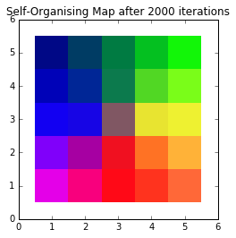
A self-organising colour map
None of those colours necessarily had to be in our dataset. By moving the 3D weight vectors to more closely match our input vectors, we’ve created a 2D colour space which clearly shows the relationship between colours. More blue colours will map to the left part of the SOM, whereas reddish colours will map to the bottom, and so on.
Other Examples
Finding a 2D colour space is a good visual way to get used to the idea of a SOM. However, there are obviously practical applications of this algorithm.
Iris Dataset
A dataset favoured by the machine learning community is Sir Ronald Fisher’s dataset of measurements of irises. There are four input dimensions: petal width, petal length, sepal width and sepal length and we could use a SOM to find similar flowers.
Applying the iris data to a SOM and then retrospectively colouring each point with their true class (to see how good the SOM was at separating the irises into their distinct categories) we get something like this:
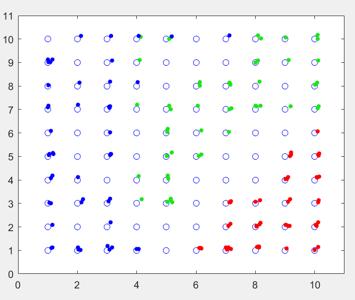
150 irises mapped onto a SOM, coloured by type
This is a 10 by 10 SOM and each of the small points is one of the irises from the dataset (with added jitter to see multiple points on a single SOM neuron). I added the colours after training, and you can quite clearly see the 3 distinct regions the SOM has divided itself into.
There are a few SOM neurons where both the green and the blue points get assigned to, and this represents the overlap between the versicolor and virginica types.
Handwritten Digits
Another application I touched on in Part 1 is trying to identify handwritten characters.
In this case, the inputs are high-dimensional – each input dimension represents the grayscale value of one pixel on a 28 by 28 image. That makes the inputs 784-dimensional (each dimension is a value between 0 and 255).
Mapping them to a 20 by 20 SOM, and again retrospectively colouring them based on their true class (a number from 0 to 9) yields this:
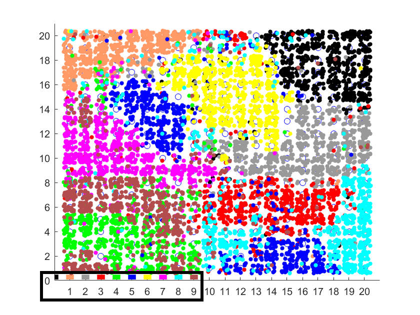
Various handwritten numbers mapped to a 2D SOM
In this case the true classes are labelled according to the colours in the bottom left.
What you can see is that the SOM has successfully divided the 2D space into regions. Despite some overlap, in most cases similar digits get mapped to the same region.
For example, the yellow region is where the 6s were mapped, and there is little overlap with other categories. Whereas in the bottom left, where the green and brown points overlap, is where the SOM was “confused” between 4s and 9s. A visual inspection of some of these handwritten characters shows that indeed many of the 4s and 9s are easily confused.
Further Reading
I hope this was a useful walkthrough on the intuition behind a SOM, and a simple Python implementation. There is a Jupyter notebook for the colour map example.
Mat Buckland’s excellent explanation and code walkthrough of SOMs was instrumental in helping me learn. My code is more or less a Python port of his C++ implementation. Reading his posts should fill in any gaps I may have not covered.