In a previous post, I used stock market data to show how prophet detects changepoints in a signal (http://pythondata.com/forecasting-time-series-data-prophet-trend-changepoints/). After publishing that article, I’ve received a few questions asking how well (or poorly) prophet can forecast the stock market so I wanted to provide a quick write-up to look at stock market forecasting with prophet.
This article highlights using prophet for forecasting the markets. You can find a jupyter notebook with the full code used in this post here.
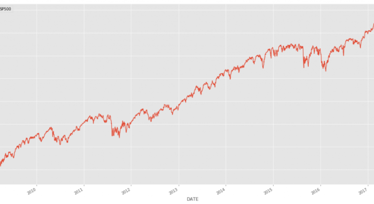
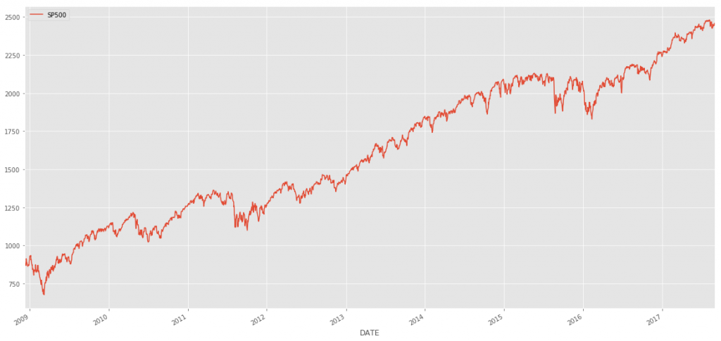
For this article, we’ll be using S&P 500 data from FRED. You can download this data into CSV format yourself or just grab a copy from the my github ‘examples’ directory here. let’s load our data and plot it.
market_df = pd.read_csv('../examples/SP500.csv', index_col='DATE', parse_dates=True)
market_df.plot()
with
Now, let’s run this data through prophet. Take a look at http://pythondata.com/forecasting-time-series-data-prophet-jupyter-notebook/ for more information on the basics of Prophet.
df = market_df.reset_index().rename(columns={'DATE':'ds', 'SP500':'y'})
df['y'] = np.log(df['y'])
model = Prophet()
model.fit(df);
future = model.make_future_dataframe(periods=365) #forecasting for 1 year from now.
forecast = model.predict(future)
And, let’s take a look at our forecast.
figure=model.plot(forecast)
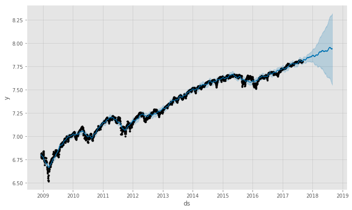
With the data that we have, it is hard to see how good/bad the forecast (blue line) is compared to the actual data (black dots). Let’s take a look at the last 800 data points (~2 years) of forecast vs actual without looking at the future forecast (because we are just interested in getting a visual of the error between actual vs forecast).
two_years = forecast.set_index('ds').join(market_df)
two_years = two_years[['SP500', 'yhat', 'yhat_upper', 'yhat_lower' ]].dropna().tail(800)
two_years['yhat']=np.exp(two_years.yhat)
two_years['yhat_upper']=np.exp(two_years.yhat_upper)
two_years['yhat_lower']=np.exp(two_years.yhat_lower)
two_years[['SP500', 'yhat']].plot()
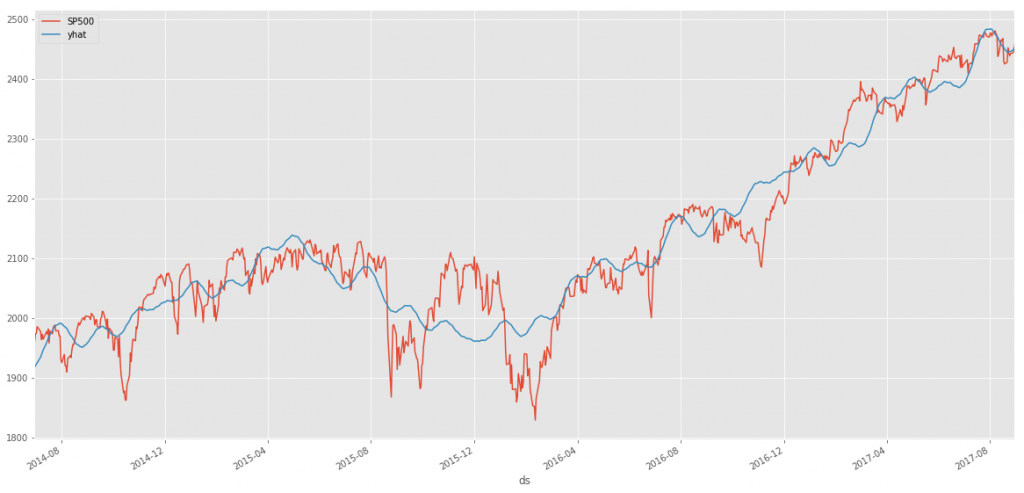
You can see from the above chart, our forecast follows the trend quite well but doesn’t seem to that great at catching the ‘volatility’ of the market. Don’t fret though…this may be a very good thing though for us if we are interested in ‘riding the trend’ rather than trying to catch peaks and dips perfectly.
Let’s take a look at a few measures of accuracy. First, we’ll look at a basic pandas dataframe describe function to see how thing slook then we’ll look at R-squared, Mean Squared Error (MSE) and Mean Absolute Error (MAE).
two_years_AE = (two_years.yhat - two_years.SP500)
print two_years_AE.describe()

count    800.000000
mean      -0.540173
std       47.568987
min     -141.265774
25%      -29.383549
50%       -1.548716
75%       25.878416
max      168.898459
dtype: float64
Those really aren’t bad numbers but they don’t really tell all of the story. Let’s take a look at a few more measures of accuracy.
Now, let’s look at R-squared using sklearn’sr2_score function:
r2_score(two_years.SP500, two_years.yhat)
We get a value of 0.91, which isn’t bad at all. I’ll take a 0.9 value in any first-go-round modeling approach.
Now, let’s look at mean squared error using sklearn’smean_squared_error function:
mean_squared_error(two_years.SP500, two_years.yhat)
We get a value of 2260.27.
And there we have it…the real pointer to this modeling technique being a bit wonky.
An MSE of 2260.28 for a model that is trying to predict the S&P500 with values between 1900 and 2500 isn’t that good (remember…for MSE, closer to zero is better) if you are trying to predict exact changes and movements up/down.
Now, let’s look at the mean absolute error (MAE) using sklearn’s mean_absolute_error function. The MAE is the measurement of absolute error between two continuous variables and can give us a much better look at error rates than the standard mean.
mean_absolute_error(two_years.SP500, two_years.yhat)
For the MAE, we get 36.18
The MAE is continuing to tell us that the forecast by prophet isn’t ideal to use this forecast in trading.
Another way to look at the usefulness of this forecast is to plot the upper and lower confidence bands of the forecast against the actuals. You can do that by plotting yhat_upper and yhat_lower.
fig, ax1 = plt.subplots()
ax1.plot(two_years.SP500)
ax1.plot(two_years.yhat)
ax1.plot(two_years.yhat_upper, color='black',  linestyle=':', alpha=0.5)
ax1.plot(two_years.yhat_lower, color='black',  linestyle=':', alpha=0.5)

ax1.set_title('Actual S&P 500 (Orange) vs S&P 500 Forecasted Upper & Lower Confidence (Black)')
ax1.set_ylabel('Price')
ax1.set_xlabel('Date')
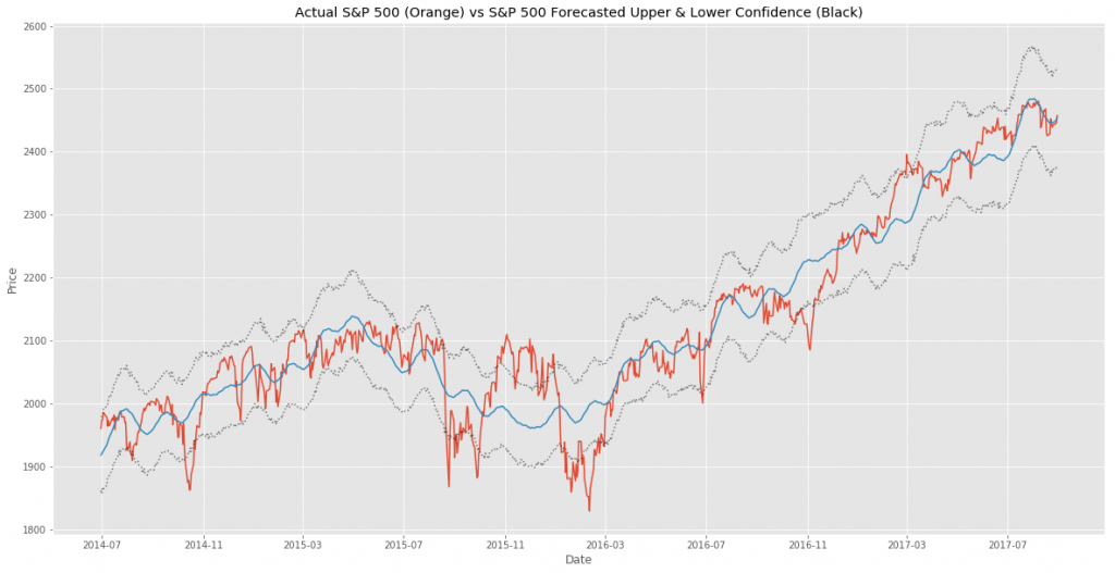
In the above chart, we can see the forecast (in blue) vs the actuals (in orange) with the upper and lower confidence bands in gray.
You can’t really tell anything quantifiable from this chart, but you can make a judgement on the value of the forecast. If you are trying to trade short-term (1 day to a few weeks) this forecast is almost useless but if you are investing with a timeframe of months to years, this forecast might provide some value to better understand the trend of the market and the forecasted trend.
Let’s go back and look at the actual forecast to see if it might tell us anything different than the forecast vs the actual data.
full_df = forecast.set_index('ds').join(market_df)
full_df['yhat']=np.exp(full_df['yhat'])

fig, ax1 = plt.subplots()
ax1.plot(full_df.SP500)
ax1.plot(full_df.yhat, color='black', linestyle=':')
ax1.fill_between(full_df.index, np.exp(full_df['yhat_upper']), np.exp(full_df['yhat_lower']), alpha=0.5, color='darkgray')
ax1.set_title('Actual S&P 500 (Orange) vs S&P 500 Forecasted (Black) with Confidence Bands')
ax1.set_ylabel('Price')
ax1.set_xlabel('Date')

L=ax1.legend() #get the legend
L.get_texts()[0].set_text('S&P 500 Actual') #change the legend text for 1st plot
L.get_texts()[1].set_text('S&P 5600 Forecasted') #change the legend text for 2nd plot
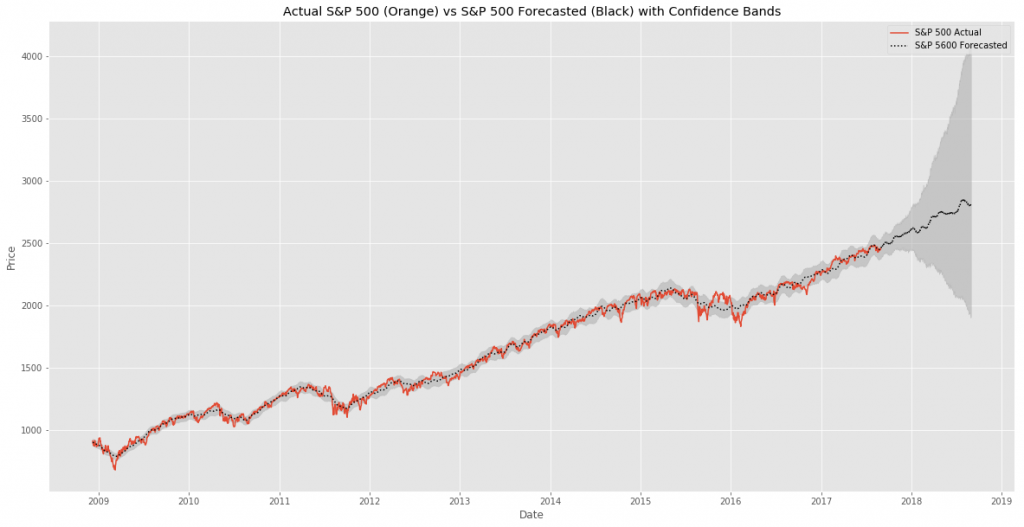
This chart is a bit easier to understand vs the default prophet chart (in my opinion at least). We can see throughout the history of the actuals vs forecast, that prophet does an OK job forecasting but has trouble with the areas when the market become very volatile.
Looking specifically at the future forecast, prophet is telling us that the market is going to continue rising and should be around 2750 at the end of the forecast period, with confidence bands stretching from 2000-ish to 4000-ish. If you show this forecast to any serious trader / investor, they’d quickly shrug it off as a terrible forecast. Anything that has a 2000 point confidence interval is worthless in the short- and long-term investing world.
That said, is there some value in prophet’s forecasting for the markets? Maybe. Perhaps a forecast looking only as a few days/weeks into the future would be much better than one that looks a year into the future. Maybe we can use the forecast on weekly or monthly data with better accuracy. Or…maybe we can use the forecast combined with other forecasts to make a better forecast. I may dig into that a bit more at some point in the future. Stay tuned.
The post Stock market forecasting with prophet appeared first on Python Data.