It is sometimes said that Python, compared to low-level languages such as C++, improves development time at the expense of runtime. Fortunately, there are a handful of ways to speed up operation runtime in Python without sacrificing ease of use. One option suited for fast numerical operations is NumPy, which deservedly bills itself as the fundamental package for scientific computing with Python.
Granted, few people would categorize something that takes 50 microseconds (fifty millionths of a second) as “slow.” However, computers might beg to differ. The runtime of an operation taking 50 microseconds (50 μs) falls under the realm of microperformance, which can loosely be defined as operations with a runtime between 1 microsecond and 1 millisecond.
Why does speed matter? The reason that microperformance is worth monitoring is that small differences in runtime become amplified with repeated function calls: an incremental 50 μs of overhead, repeated over 1 million function calls, translates to 50 seconds of incremental runtime.
When it comes to computation, there are really three concepts that lend NumPy its power:
- Vectorization
- Broadcasting
- Indexing
In this tutorial, you’ll see step by step how to take advantage of vectorization and broadcasting, so that you can use NumPy to its full capacity. While you will use some indexing in practice here, NumPy’s complete indexing schematics, which extend Python’s slicing syntax, are their own beast. If you’re looking to read more on NumPy indexing, grab some coffee and head to the Indexing section in the NumPy docs.
Free Bonus: Click here to get access to a free NumPy Resources Guide that points you to the best tutorials, videos, and books for improving your NumPy skills.
Getting into Shape: Intro to NumPy Arrays
The fundamental object of NumPy is its ndarray (or numpy.array), an n-dimensional array that is also present in some form in array-oriented languages such as Fortran 90, R, and MATLAB, as well as predecessors APL and J.
Let’s start things off by forming a 3-dimensional array with 36 elements:
>>> import numpy as np

>>> arr = np.arange(36).reshape(3, 4, 3)
>>> arr
array([[[ 0,  1,  2],
        [ 3,  4,  5],
        [ 6,  7,  8],
        [ 9, 10, 11]],

       [[12, 13, 14],
        [15, 16, 17],
        [18, 19, 20],
        [21, 22, 23]],

       [[24, 25, 26],
        [27, 28, 29],
        [30, 31, 32],
        [33, 34, 35]]])
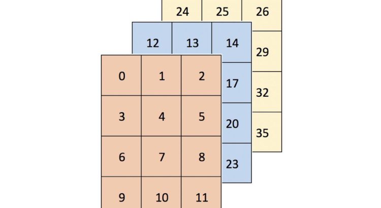
Picturing high-dimensional arrays in two dimensions can be difficult. One intuitive way to think about an array’s shape is to simply “read it from left to right.” arr is a 3 by 4 by 3 array:
>>> arr.shape
(3, 4, 3)
Visually, arr could be thought of as a container of three 4×3 grids (or a rectangular prism) and would look like this:
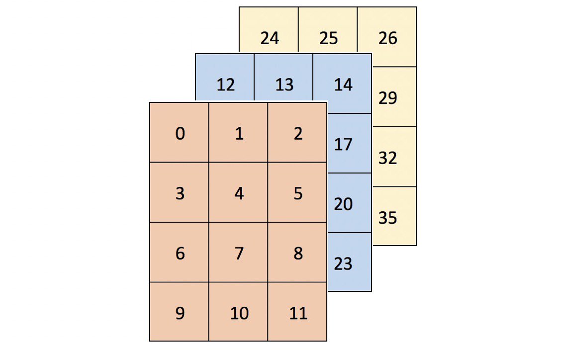
Higher dimensional arrays can be tougher to picture, but they will still follow this “arrays within an array” pattern.
Where might you see data with greater than two dimensions?
- Panel data can be represented in three dimensions. Data that tracks attributes of a cohort (group) of individuals over time could be structured as
(respondents, dates, attributes). The 1979 National Longitudinal Survey of Youth follows 12,686 respondents over 27 years. Assuming that you have ~500 directly asked or derived data points per individual, per year, this data would have shape(12686, 27, 500)for a total of 177,604,000 data points. - Color-image data for multiple images is typically stored in four dimensions. Each image is a three-dimensional array of
(height, width, channels), where the channels are usually red, green, and blue (RGB) values. A collection of images is then just(image_number, height, width, channels). One thousand 256×256 RGB images would have shape(1000, 256, 256, 3). (An extended representation is RGBA, where the A–alpha–denotes the level of opacity.)
For more detail on real-world examples of high-dimensional data, see Chapter 2 of François Chollet’s Deep Learning with Python.
What is Vectorization?
Vectorization is a powerful ability within NumPy to express operations as occurring on entire arrays rather than their individual elements. Here’s a concise definition from Wes McKinney:
This practice of replacing explicit loops with array expressions is commonly referred to as vectorization. In general, vectorized array operations will often be one or two (or more) orders of magnitude faster than their pure Python equivalents, with the biggest impact [seen] in any kind of numerical computations. [source]
When looping over an array or any data structure in Python, there’s a lot of overhead involved. Vectorized operations in NumPy delegate the looping internally to highly optimized C and Fortran functions, making for cleaner and faster Python code.
Counting: Easy as 1, 2, 3…
As an illustration, consider a 1-dimensional vector of True and False for which you want to count the number of “False to True” transitions in the sequence:
>>> np.random.seed(444)

>>> x = np.random.choice([False, True], size=100000)
>>> x
array([ True, False,  True, ...,  True, False,  True])
With a Python for-loop, one way to do this would be to evaluate, in pairs, the truth value of each element in the sequence along with the element that comes right after it:
>>> def count_transitions(x) -> int:
...     count = 0
...     for i, j in zip(x[:-1], x[1:]):
...         if j and not i:
...             count += 1
...     return count
...
>>> count_transitions(x)
24984
In vectorized form, there’s no explicit for-loop or direct reference to the individual elements:
>>> np.count_nonzero(x[:-1] < x[1:])
24984
How do these two equivalent functions compare in terms of performance? In this particular case, the vectorized NumPy call wins out by a factor of about 70 times:
>>> from timeit import timeit
>>> setup = 'from __main__ import count_transitions, x; import numpy as np'
>>> num = 1000
>>> t1 = timeit('count_transitions(x)', setup=setup, number=num)
>>> t2 = timeit('np.count_nonzero(x[:-1] < x[1:])', setup=setup, number=num)
>>> print('Speed difference: {:0.1f}x'.format(t1 / t2))
Speed difference: 71.0x
Technical Detail: Another term is vector processor, which is related to a computer’s hardware. When I speak about vectorization here, I’m referring to concept of replacing explicit for-loops with array expressions, which in this case can then be computed internally with a low-level language.
Buy Low, Sell High
Here’s another example to whet your appetite. Consider the following classic technical interview problem:
Given a stock’s price history as a sequence, and assuming that you are only allowed to make one purchase and one sale, what is the maximum profit that can be obtained? For example, given
prices = (20, 18, 14, 17, 20, 21, 15), the max profit would be 7, from buying at 14 and selling at 21.
(To all of you finance people: no, short-selling is not allowed.)
There is a solution with n-squared time complexity that consists of taking every combination of two prices where the second price “comes after” the first and determining the maximum difference.
However, there is also an O(n) solution that consists of iterating through the sequence just once and finding the difference between each price and a running minimum. It goes something like this:
>>> def profit(prices):
...     max_px = 0
...     min_px = prices[0]
...     for px in prices[1:]:
...         min_px = min(min_px, px)
...         max_px = max(px - min_px, max_px)
...     return max_px

>>> prices = (20, 18, 14, 17, 20, 21, 15)
>>> profit(prices)
7
Can this be done in NumPy? You bet. But first, let’s build a quasi-realistic example:
# Create mostly NaN array with a few 'turning points' (local min/max).
>>> prices = np.full(100, fill_value=np.nan)
>>> prices[[0, 25, 60, -1]] = [80., 30., 75., 50.]

# Linearly interpolate the missing values and add some noise.
>>> x = np.arange(len(prices))
>>> is_valid = ~np.isnan(prices)
>>> prices = np.interp(x=x, xp=x[is_valid], fp=prices[is_valid])
>>> prices += np.random.randn(len(prices)) * 2
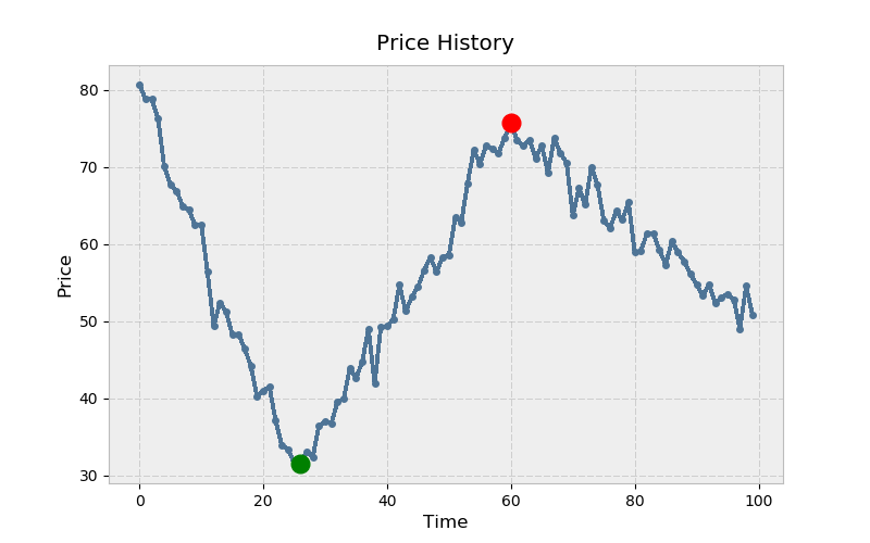
Here’s what this looks like with matplotlib. The adage is to buy low (green) and sell high (red):
>>> import matplotlib.pyplot as plt

# Warning! This isn't a fully correct solution, but it works for now.
# If the absolute min came after the absolute max, you'd have trouble.
>>> mn = np.argmin(prices)
>>> mx = mn + np.argmax(prices[mn:])
>>> kwargs = {'markersize': 12, 'linestyle': ''}

>>> fig, ax = plt.subplots()
>>> ax.plot(prices)
>>> ax.set_title('Price History')
>>> ax.set_xlabel('Time')
>>> ax.set_ylabel('Price')
>>> ax.plot(mn, prices[mn], color='green', **kwargs)
>>> ax.plot(mx, prices[mx], color='red', **kwargs)
What does the NumPy implementation look like? While there is no np.cummin() “directly,” NumPy’s universal functions (ufuncs) all have an accumulate() method that does what its name implies:
>>> cummin = np.minimum.accumulate
Extending the logic from the pure-Python example, you can find the difference between each price and a running minimum (element-wise), and then take the max of this sequence:
>>> def profit_with_numpy(prices):
...     """Price minus cumulative minimum price, element-wise."""
...     prices = np.asarray(prices)
...     return np.max(prices - cummin(prices))

>>> profit_with_numpy(prices)
44.2487532293278
>>> np.allclose(profit_with_numpy(prices), profit(prices))
True
How do these two operations, which have the same theoretical time complexity, compare in actual runtime? First, let’s take a longer sequence. (This doesn’t necessarily need to be a time series of stock prices at this point.)
>>> seq = np.random.randint(0, 100, size=100000)
>>> seq
array([ 3, 23,  8, 67, 52, 12, 54, 72, 41, 10, ..., 46,  8, 90, 95, 93,
       28, 24, 88, 24, 49])
Now, for a somewhat unfair comparison:
>>> setup = ('from __main__ import profit_with_numpy, profit, seq;'
...          ' import numpy as np')
>>> num = 250
>>> pytime = timeit('profit(seq)', setup=setup, number=num)
>>> nptime = timeit('profit_with_numpy(seq)', setup=setup, number=num)
>>> print('Speed difference: {:0.1f}x'.format(pytime / nptime))
Speed difference: 76.0x
Above, treating profit_with_numpy() as pseudocode (without considering NumPy’s underlying mechanics), there are actually three passes through a sequence:
cummin(prices)has O(n) time complexityprices - cummin(prices)is O(n)max(...)is O(n)
This reduces to O(n), because O(3n) reduces to just O(n)–the n “dominates” as n approaches infinity.
Therefore, these two functions have equivalent worst-case time complexity. (Although, as a side note, the NumPy function comes with significantly more space complexity.) But that is probably the least important takeaway here. One lesson is that, while theoretical time complexity is an important consideration, runtime mechanics can also play a big role. Not only can NumPy delegate to C, but with some element-wise operations and linear algebra, it can also take advantage of computing within multiple threads. But there are a lot of factors at play here, including the underlying library used (BLAS/LAPACK/Atlas), and those details are for a whole ‘nother article entirely.
Intermezzo: Understanding Axes Notation
In NumPy, an axis refers to a single dimension of a multidimensional array:
>>> arr = np.array([[1, 2, 3],
...                 [10, 20, 30]])
>>> arr.sum(axis=0)
array([11, 22, 33])
>>> arr.sum(axis=1)
array([ 6, 60])
The terminology around axes and the way in which they are described can be a bit unintuitive. In the documentation for Pandas (a library built on top of NumPy), you may frequently see something like:
axis : {'index' (0), 'columns' (1)}
You could argue that, based on this description, the results above should be “reversed.” However, the key is that axis refers to the axis along which a function gets called. This is well articulated by Jake VanderPlas:
The way the axis is specified here can be confusing to users coming from other languages. The axis keyword specifies the dimension of the array that will be collapsed, rather than the dimension that will be returned. So, specifying
axis=0means that the first axis will be collapsed: for two-dimensional arrays, this means that values within each column will be aggregated. [source]
In other words, summing an array for axis=0 collapses the rows of the array with a column-wise computation.
With this distinction in mind, let’s move on to explore the concept of broadcasting.
Broadcasting
Broadcasting is another important NumPy abstraction. You’ve already seen that operations between two NumPy arrays (of equal size) operate element-wise:
>>> a = np.array([1.5, 2.5, 3.5])
>>> b = np.array([10., 5., 1.])
>>> a / b
array([0.15, 0.5 , 3.5 ])
But, what about unequally sized arrays? This is where broadcasting comes in:
The term broadcasting describes how NumPy treats arrays with different shapes during arithmetic operations. Subject to certain constraints, the smaller array is “broadcast” across the larger array so that they have compatible shapes. Broadcasting provides a means of vectorizing array operations so that looping occurs in C instead of Python. [source]
The way in which broadcasting is implemented can become tedious when working with more than two arrays. However, if there are just two arrays, then their ability to be broadcasted can be described with two short rules:
When operating on two arrays, NumPy compares their shapes element-wise. It starts with the trailing dimensions and works its way forward. Two dimensions are compatible when:
- they are equal, or
- one of them is 1
That’s all there is to it.
Let’s take a case where we want to subtract each column-wise mean of an array, element-wise:
>>> sample = np.random.normal(loc=[2., 20.], scale=[1., 3.5],
...                           size=(3, 2))
>>> sample
array([[ 1.816 , 23.703 ],
       [ 2.8395, 12.2607],
       [ 3.5901, 24.2115]])
In statistical jargon, sample consists of two samples (the columns) drawn independently from two populations with means of 2 and 20, respectively. The column-wise means should approximate the population means (albeit roughly, because the sample is small):
>>> mu = sample.mean(axis=0)
>>> mu
array([ 2.7486, 20.0584])
Now, subtracting the column-wise means is straightforward because broadcasting rules check out:
>>> print('sample:', sample.shape, '| means:', mu.shape)
sample: (3, 2) | means: (2,)

>>> sample - mu
array([[-0.9325,  3.6446],
       [ 0.091 , -7.7977],
       [ 0.8416,  4.1531]])
Here’s an illustration of subtracting out column-wise means, where a smaller array is “stretched” so that it is subtracted from each row of the larger array:
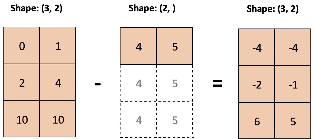
Technical Detail: The smaller-sized array or scalar is not literally stretched in memory: it is the computation itself that is repeated.
This extends to standardizing each column as well, making each cell a z-score relative to its respective column:
>>> (sample - sample.mean(axis=0)) / sample.std(axis=0)
array([[-1.2825,  0.6605],
       [ 0.1251, -1.4132],
       [ 1.1574,  0.7527]])
However, what if you want to subtract out, for some reason, the row-wise minimums? You’ll run into a bit of trouble:
>>> sample - sample.min(axis=1)
ValueError: operands could not be broadcast together with shapes (3,2) (3,)
The problem here is that the smaller array, in its current form, cannot be “stretched” to be shape-compatible with sample. You actually need to expand its dimensionality to meet the broadcasting rules above:
>>> sample.min(axis=1)[:, None]  # 3 minimums across 3 rows
array([[1.816 ],
       [2.8395],
       [3.5901]])

>>> sample - sample.min(axis=1)[:, None]
array([[ 0.    , 21.887 ],
       [ 0.    ,  9.4212],
       [ 0.    , 20.6214]])
Note: [:, None] is a means by which to expand the dimensionality of an array, to create an axis of length one. np.newaxis is an alias for None.
There are some significantly more complex cases, too. Here’s a more rigorous definition of when any arbitrary number of arrays of any shape can be broadcast together:
A set of arrays is called “broadcastable” to the same shape if the following rules produce a valid result, meaning one of the following is true:
The arrays all have exactly the same shape.
The arrays all have the same number of dimensions, and the length of each dimension is either a common length or 1.
The arrays that have too few dimensions can have their shapes prepended with a dimension of length 1 to satisfy property #2.
[source]
This is easier to walk through step by step. Let’s say you have the following four arrays:
>>> a = np.sin(np.arange(10)[:, None])
>>> b = np.random.randn(1, 10)
>>> c = np.full_like(a, 10)
>>> d = 8
Before checking shapes, NumPy first converts scalars to arrays with one element:
>>> arrays = [np.atleast_1d(arr) for arr in (a, b, c, d)]
>>> for arr in arrays:
...     print(arr.shape)
...
(10, 1)
(1, 10)
(10, 1)
(1,)
Now we can check criterion #1. If all of the arrays have the same shape, a set of their shapes will condense down to one element, because the set() constructor effectively drops duplicate items from its input. This criterion is clearly not met:
>>> len(set(arr.shape for arr in arrays)) == 1
False
The first part of criterion #2 also fails, meaning the entire criterion fails:
>>> len(set((arr.ndim) for arr in arrays)) == 1
False
The final criterion is a bit more involved:
The arrays that have too few dimensions can have their shapes prepended with a dimension of length 1 to satisfy property #2.
To codify this, you can first determine the dimensionality of the highest-dimension array and then prepend ones to each shape tuple until all are of equal dimension:
>>> maxdim = max(arr.ndim for arr in arrays)  # Maximum dimensionality
>>> shapes = np.array([(1,) * (maxdim - arr.ndim) + arr.shape
...                    for arr in arrays])
>>> shapes
array([[10,  1],
       [ 1, 10],
       [10,  1],
       [ 1,  1]])
Finally, you need to test that the length of each dimension is either (drawn from) a common length, or 1. A trick for doing this is to first mask the array of “shape-tuples” in places where it equals one. Then, you can check if the peak-to-peak (np.ptp()) column-wise differences are all zero:
>>> masked = np.ma.masked_where(shapes == 1, shapes)
>>> np.all(masked.ptp(axis=0) == 0)  # ptp: max - min
True
Encapsulated in a single function, this logic looks like this:
>>> def can_broadcast(*arrays) -> bool:
...     arrays = [np.atleast_1d(arr) for arr in arrays]
...     if len(set(arr.shape for arr in arrays)) == 1:
...         return True
...     if len(set((arr.ndim) for arr in arrays)) == 1:
...         return True
...     maxdim = max(arr.ndim for arr in arrays)
...     shapes = np.array([(1,) * (maxdim - arr.ndim) + arr.shape
...                        for arr in arrays])
...     masked = np.ma.masked_where(shapes == 1, shapes)
...     return np.all(masked.ptp(axis=0) == 0)
...
>>> can_broadcast(a, b, c, d)
True
Luckily, you can take a shortcut and use np.broadcast() for this sanity-check, although it’s not explicitly designed for this purpose:
>>> def can_broadcast(*arrays) -> bool:
...     try:
...         np.broadcast(*arrays)
...         return True
...     except ValueError:
...         return False
...
>>> can_broadcast(a, b, c, d)
True
For those interested in digging a little deeper, PyArray_Broadcast is the underlying C function that encapsulates broadcasting rules.
Array Programming in Action: Examples
In the following 3 examples, you’ll put vectorization and broadcasting to work with some real-world applications.
Clustering Algorithms
Machine learning is one domain that can frequently take advantage of vectorization and broadcasting. Let’s say that you have the vertices of a triangle (each row is an x, y coordinate):
>>> tri = np.array([[1, 1],
...                 [3, 1],
...                 [2, 3]])
The centroid of this “cluster” is an (x, y) coordinate that is the arithmetic mean of each column:
>>> centroid = tri.mean(axis=0)
>>> centroid
array([2.    , 1.6667])
It’s helpful to visualize this:
>>> trishape = plt.Polygon(tri, edgecolor='r', alpha=0.2, lw=5)
>>> _, ax = plt.subplots(figsize=(4, 4))
>>> ax.add_patch(trishape)
>>> ax.set_ylim([.5, 3.5])
>>> ax.set_xlim([.5, 3.5])
>>> ax.scatter(*centroid, color='g', marker='D', s=70)
>>> ax.scatter(*tri.T, color='b',  s=70)

Many clustering algorithms make use of Euclidean distances of a collection of points, either to the origin or relative to their centroids.
In Cartesian coordinates, the Euclidean distance between points p and q is:
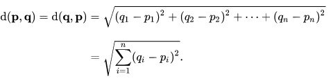
So for the set of coordinates in tri from above, the Euclidean distance of each point from the origin (0, 0) would be:
>>> np.sum(tri**2, axis=1) ** 0.5  # Or: np.sqrt(np.sum(np.square(tri), 1))
array([1.4142, 3.1623, 3.6056])
You may recognize that we are really just finding Euclidean norms:
>>> np.linalg.norm(tri, axis=1)
array([1.4142, 3.1623, 3.6056])
Instead of referencing the origin, you could also find the norm of each point relative to the triangle’s centroid:
>>> np.linalg.norm(tri - centroid, axis=1)
array([1.2019, 1.2019, 1.3333])
Finally, let’s take this one step further: let’s say that you have a 2d array X and a 2d array of multiple (x, y) “proposed” centroids. Algorithms such as K-Means clustering work by randomly assigning initial “proposed” centroids, then reassigning each data point to its closest centroid. From there, new centroids are computed, with the algorithm converging on a solution once the re-generated labels (an encoding of the centroids) are unchanged between iterations. A part of this iterative process requires computing the Euclidean distance of each point from each centroid:
>>> X = np.repeat([[5, 5], [10, 10]], [5, 5], axis=0)
>>> X = X + np.random.randn(*X.shape)  # 2 distinct "blobs"
>>> centroids = np.array([[5, 5], [10, 10]])

>>> X
array([[ 3.3955,  3.682 ],
       [ 5.9224,  5.785 ],
       [ 5.9087,  4.5986],
       [ 6.5796,  3.8713],
       [ 3.8488,  6.7029],
       [10.1698,  9.2887],
       [10.1789,  9.8801],
       [ 7.8885,  8.7014],
       [ 8.6206,  8.2016],
       [ 8.851 , 10.0091]])

>>> centroids
array([[ 5,  5],
       [10, 10]])
In other words, we want to answer the question, to which centroid does each point within X belong? We need to do some reshaping to enable broadcasting here, in order to calculate the Euclidean distance between each point in X and each point in centroids:
>>> centroids[:, None]
array([[[ 5,  5]],

       [[10, 10]]])

>>> centroids[:, None].shape
(2, 1, 2)
This enables us to cleanly subtract one array from another using a combinatoric product of their rows:
>>> np.linalg.norm(X - centroids[:, None], axis=2).round(2)
array([[2.08, 1.21, 0.99, 1.94, 2.06, 6.72, 7.12, 4.7 , 4.83, 6.32],
       [9.14, 5.86, 6.78, 7.02, 6.98, 0.73, 0.22, 2.48, 2.27, 1.15]])
In other words, the shape of X - centroids[:, None] is (2, 10, 2), essentially representing two stacked arrays that are each the size of X. Next, we want the label (index number) of each closest centroid, finding the minimum distance on the 0th axis from the array above:
>>> np.argmin(np.linalg.norm(X - centroids[:, None], axis=2), axis=0)
array([0, 0, 0, 0, 0, 1, 1, 1, 1, 1])
You can put all this together in functional form:
>>> def get_labels(X, centroids) -> np.ndarray:
...     return np.argmin(np.linalg.norm(X - centroids[:, None], axis=2),
...                      axis=0)
>>> labels = get_labels(X, centroids)
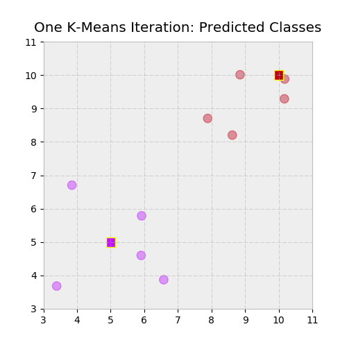
Let’s inspect this visually, plotting both the two clusters and their assigned labels with a color-mapping:
>>> c1, c2 = ['#bc13fe', '#be0119']  # https://xkcd.com/color/rgb/
>>> llim, ulim  = np.trunc([X.min() * 0.9, X.max() * 1.1])

>>> _, ax = plt.subplots(figsize=(5, 5))
>>> ax.scatter(*X.T, c=np.where(labels, c2, c1), alpha=0.4, s=80)
>>> ax.scatter(*centroids.T, c=[c1, c2], marker='s', s=95,
...            edgecolor='yellow')
>>> ax.set_ylim([llim, ulim])
>>> ax.set_xlim([llim, ulim])
>>> ax.set_title('One K-Means Iteration: Predicted Classes')
Amortization Tables
Vectorization has applications in finance as well.
Given an annualized interest rate, payment frequency (times per year), initial loan balance, and loan term, you can create an amortization table with monthly loan balances and payments, in a vectorized fashion. Let’s set some scalar constants first:
>>> freq = 12     # 12 months per year
>>> rate = .0675  # 6.75% annualized
>>> nper = 30     # 30 years
>>> pv = 200000   # Loan face value

>>> rate /= freq  # Monthly basis
>>> nper *= freq  # 360 months
NumPy comes preloaded with a handful of financial functions that, unlike their Excel cousins, are capable of producing vector outputs.
The debtor (or lessee) pays a constant monthly amount that is composed of a principal and interest component. As the outstanding loan balance declines, the interest portion of the total payment declines with it.
>>> periods = np.arange(1, nper + 1, dtype=int)
>>> principal = np.ppmt(rate, periods, nper, pv)
>>> interest = np.ipmt(rate, periods, nper, pv)
>>> pmt = principal + interest  # Or: pmt = np.pmt(rate, nper, pv)
Next, you’ll need to calculate a monthly balance, both before and after that month’s payment, which can be defined as the future value of the original balance minus the future value of an annuity (a stream of payments), using a discount factor d:
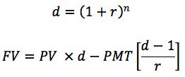
Functionally, this looks like:
>>> def balance(pv, rate, nper, pmt) -> np.ndarray:
...     d = (1 + rate) ** nper  # Discount factor
...     return pv * d - pmt * (d - 1) / rate
Finally, you can drop this into a tabular format with a Pandas DataFrame. Be careful with signs here. PMT is an outflow from the perspective of the debtor.
>>> import pandas as pd

>>> cols = ['beg_bal', 'prin', 'interest', 'end_bal']
>>> data = [balance(pv, rate, periods - 1, -pmt),
...         principal,
...         interest,
...         balance(pv, rate, periods, -pmt)]

>>> table = pd.DataFrame(data, columns=periods, index=cols).T
>>> table.index.name = 'month'

>>> with pd.option_context('display.max_rows', 6):
...     # Note: Using floats for $$ in production-level code = bad
...     print(table.round(2))
...
         beg_bal     prin  interest    end_bal
month
1      200000.00  -172.20  -1125.00  199827.80
2      199827.80  -173.16  -1124.03  199654.64
3      199654.64  -174.14  -1123.06  199480.50
...          ...      ...       ...        ...
358      3848.22 -1275.55    -21.65    2572.67
359      2572.67 -1282.72    -14.47    1289.94
360      1289.94 -1289.94     -7.26      -0.00
At the end of year 30, the loan is paid off:
>>> final_month = periods[-1]
>>> np.allclose(table.loc[final_month, 'end_bal'], 0)
True
Note: While using floats to represent money can be useful for concept illustration in a scripting environment, using Python floats for financial calculations in a production environment might cause your calculation to be a penny or two off in some cases.
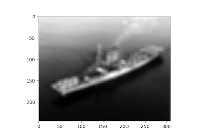
Image Feature Extraction
In one final example, we’ll work with an October 1941 image of the USS Lexington (CV-2), the wreck of which was discovered off the coast of Australia in March 2018. First, we can map the image into a NumPy array of its pixel values:
>>> from skimage import io

>>> url = ('https://www.history.navy.mil/bin/imageDownload?image=/'
...        'content/dam/nhhc/our-collections/photography/images/'
...        '80-G-410000/80-G-416362&rendition=cq5dam.thumbnail.319.319.png')
>>> img = io.imread(url, as_grey=True)

>>> fig, ax = plt.subplots()
>>> ax.imshow(img, cmap='gray')
>>> ax.grid(False)
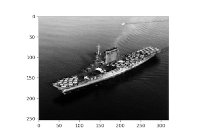
For simplicity’s sake, the image is loaded in grayscale, resulting in a 2d array of 64-bit floats rather than a 3-dimensional MxNx4 RGBA array, with lower values denoting darker spots:
>>> img.shape
(254, 319)

>>> img.min(), img.max()
(0.027450980392156862, 1.0)

>>> img[0, :10]  # First ten cells of the first row
array([0.8078, 0.7961, 0.7804, 0.7882, 0.7961, 0.8078, 0.8039, 0.7922,
       0.7961, 0.7961])
>>> img[-1, -10:]  # Last ten cells of the last row
array([0.0784, 0.0784, 0.0706, 0.0706, 0.0745, 0.0706, 0.0745, 0.0784,
       0.0784, 0.0824])
One technique commonly employed as an intermediary step in image analysis is patch extraction. As the name implies, this consists of extracting smaller overlapping sub-arrays from a larger array and can be used in cases where it is advantageous to “denoise” or blur an image.
This concept extends to other fields, too. For example, you’d be doing something similar by taking “rolling” windows of a time series with multiple features (variables). It’s even useful for building Conway’s Game of Life. (Although, convolution with a 3×3 kernel is a more direct approach.)
Here, we will find the mean of each overlapping 10×10 patch within img. Taking a miniature example, the first 3×3 patch array in the top-left corner of img would be:
>>> img[:3, :3]
array([[0.8078, 0.7961, 0.7804],
       [0.8039, 0.8157, 0.8078],
       [0.7882, 0.8   , 0.7961]])

>>> img[:3, :3].mean()
0.7995642701525054
The pure-Python approach to creating sliding patches would involve a nested for-loop. You’d need to consider that the starting index of the right-most patches will be at index n - 3 + 1, where n is the width of the array. In other words, if you were extracting 3×3 patches from a 10×10 array called arr, the last patch taken would be from arr[7:10, 7:10]. Also keep in mind that Python’s range() does not include its stop parameter:
>>> size = 10
>>> m, n = img.shape
>>> mm, nn = m - size + 1, n - size + 1
>>>
>>> patch_means = np.empty((mm, nn))
>>> for i in range(mm):
...     for j in range(nn):
...         patch_means[i, j] = img[i: i+size, j: j+size].mean()

>>> fig, ax = plt.subplots()
>>> ax.imshow(patch_means, cmap='gray')
>>> ax.grid(False)
With this loop, you’re performing a lot of Python calls.
An alternative that will be scalable to larger RGB or RGBA images is NumPy’s stride_tricks.
An instructive first step is to visualize, given the patch size and image shape, what a higher-dimensional array of patches would look like. We have a 2d array img with shape (254, 319)and a (10, 10) 2d patch. This means our output shape (before taking the mean of each “inner” 10×10 array) would be:
>>> shape = (img.shape[0] - size + 1, img.shape[1] - size + 1, size, size)
>>> shape
(245, 310, 10, 10)
You also need to specify the strides of the new array. An array’s strides is a tuple of bytes to jump in each dimension when moving along the array. Each pixel in img is a 64-bit (8-byte) float, meaning the total image size is 254 x 319 x 8 = 648,208 bytes.
>>> img.dtype
dtype('float64')

>>> img.nbytes
648208
Internally, img is kept in memory as one contiguous block of 648,208 bytes. strides is hence a sort of “metadata”-like attribute that tells us how many bytes we need to jump ahead to move to the next position along each axis. We move in blocks of 8 bytes along the rows but need to traverse 8 x 319 = 2,552 bytes to move “down” from one row to another.
>>> img.strides
(2552, 8)
In our case, the strides of the resulting patches will just repeat the strides of img twice:
>>> strides = 2 * img.strides
>>> strides
(2552, 8, 2552, 8)
Now, let’s put these pieces together with NumPy’s stride_tricks:
>>> from numpy.lib import stride_tricks

>>> patches = stride_tricks.as_strided(img, shape=shape, strides=strides)
>>> patches.shape
(245, 310, 10, 10)
Here’s the first 10×10 patch:
>>> patches[0, 0].round(2)
array([[0.81, 0.8 , 0.78, 0.79, 0.8 , 0.81, 0.8 , 0.79, 0.8 , 0.8 ],
       [0.8 , 0.82, 0.81, 0.79, 0.79, 0.79, 0.78, 0.81, 0.81, 0.8 ],
       [0.79, 0.8 , 0.8 , 0.79, 0.8 , 0.8 , 0.82, 0.83, 0.79, 0.81],
       [0.8 , 0.79, 0.81, 0.81, 0.8 , 0.8 , 0.78, 0.76, 0.8 , 0.79],
       [0.78, 0.8 , 0.8 , 0.78, 0.8 , 0.79, 0.78, 0.78, 0.79, 0.79],
       [0.8 , 0.8 , 0.78, 0.78, 0.78, 0.8 , 0.8 , 0.8 , 0.81, 0.79],
       [0.78, 0.77, 0.78, 0.76, 0.77, 0.8 , 0.8 , 0.77, 0.8 , 0.8 ],
       [0.79, 0.76, 0.77, 0.78, 0.77, 0.77, 0.79, 0.78, 0.77, 0.76],
       [0.78, 0.75, 0.76, 0.76, 0.73, 0.75, 0.78, 0.76, 0.77, 0.77],
       [0.78, 0.79, 0.78, 0.78, 0.78, 0.78, 0.77, 0.76, 0.77, 0.77]])
The last step is tricky. To get a vectorized mean of each inner 10×10 array, we need to think carefully about the dimensionality of what we have now. The result should collapse the last two dimensions so that we’re left with a single 245×310 array.
One (suboptimal) way would be to reshape patches first, flattening the inner 2d arrays to length-100 vectors, and then computing the mean on the final axis:
>>> veclen = size ** 2
>>> patches.reshape(*patches.shape[:2], veclen).mean(axis=-1).shape
(245, 310)
However, you can also specify axis as a tuple, computing a mean over the last two axes, which should be more efficient than reshaping:
>>> patches.mean(axis=(-1, -2)).shape
(245, 310)
Let’s make sure this checks out by comparing equality to our looped version. It does:
>>> strided_means = patches.mean(axis=(-1, -2))
>>> np.allclose(patch_means, strided_means)
True
If the concept of strides has you drooling, don’t worry: Scikit-Learn has already embedded this entire process nicely within its feature_extraction module.
A Parting Thought: Don’t Over-Optimize
In this article, we discussed optimizing runtime by taking advantage of array programming in NumPy. When you are working with large datasets, it’s important to be mindful of microperformance.
However, there is a subset of cases where avoiding a native Python for-loop isn’t possible. As Donald Knuth advised, “Premature optimization is the root of all evil.” Programmers may incorrectly predict where in their code a bottleneck will appear, spending hours trying to fully vectorize an operation that would result in a relatively insignificant improvement in runtime.
There’s nothing wrong with for-loops sprinkled here and there. Often, it can be more productive to think instead about optimizing the flow and structure of the entire script at a higher level of abstraction.
More Resources
Free Bonus: Click here to get access to a free NumPy Resources Guide that points you to the best tutorials, videos, and books for improving your NumPy skills.
NumPy Documentation:
- What is NumPy?
- Broadcasting
- Universal functions
- NumPy for MATLAB Users
- The complete NumPy Reference index
Books:
- Travis Oliphant’s Guide to NumPy, 2nd ed. (Travis is the primary creator of NumPy)
- Chapter 2 (“Introduction to NumPy”) of Jake VanderPlas’ Python Data Science Handbook
- Chapter 4 (“NumPy Basics”) and Chapter 12 (“Advanced NumPy”) of Wes McKinney’s Python for Data Analysis 2nd ed.
- Chapter 2 (“The Mathematical Building Blocks of Neural Networks”) from François Chollet’s Deep Learning with Python
- Robert Johansson’s Numerical Python
- Ivan Idris: Numpy Beginner’s Guide, 3rd ed.
Other Resources:
- Wikipedia: Array Programming
- SciPy Lecture Notes: Basic and Advanced NumPy
- EricsBroadcastingDoc: Array Broadcasting in NumPy
- SciPy Cookbook: Views versus copies in NumPy
- Nicolas Rougier: From Python to Numpy and 100 NumPy Exercises
- TensorFlow docs: Broadcasting Semantics
- Theano docs: Broadcasting
- Eli Bendersky: Broadcasting Arrays in Numpy
[ Improve Your Python With 🐍 Python Tricks 💌 – Get a short & sweet Python Trick delivered to your inbox every couple of days. >> Click here to learn more and see examples ]