Learn three data manipulation techniques with Pandas in this guest post by Harish Garg, a software developer and data analyst, and the author of Mastering Exploratory Analysis with pandas.
Modifying a Pandas DataFrame Using the inplace Parameter
In this section, you’ll learn how to modify a DataFrame using the inplace parameter. You’ll first read a real dataset into Pandas. You’ll then see how the inplace parameter impacts a method execution’s end result. You’ll also execute methods with and without the inplace parameter to demonstrate the effect of inplace.
Start by importing the Pandas module into your Jupyter notebook, as follows:
import pandas as pd
Then read your dataset:
top_movies = pd.read_csv('data-movies-top-grossing.csv', sep=',')
- See the Pandas DataFrame Tutorial to learn more about reading CSV files.
Since it’s a CSV file, you’ll have to use Pandas’ read_csv function for this. Now that you have read your dataset into a DataFrame, it’s time to take a look at a few of the records:
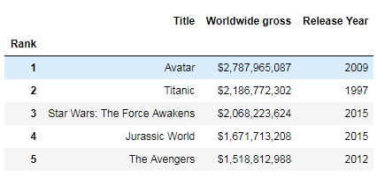
top_movies
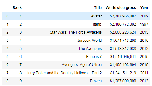
The data you’re using is from Wikipedia; it’s the cross annex data for top movies worldwide to date. Most Pandas DataFrame methods return a new DataFrame. However, you may want to use a method to modify the original DataFrame itself.
This is where the inplace parameter is useful. Try calling a method on a DataFrame without the inplace parameter to see how it works in the code:
top_movies.set_index('Rank').head()
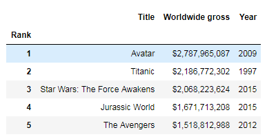
Here, you’re setting one of the columns as the index for your DataFrame. You can see that the index has been set in the memory. Now check to see if it has modified the original DataFrame or not:
top_movies.head()
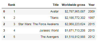
As you can see, there’s no change in the original DataFrame. The set_index method only created the change in a completely new DataFrame in memory, which you could have saved in a new DataFrame. Now see how it works when you pass the inplace parameter:
top_movies.set_index('Rank', inplace=True)
Pass inplace=True to the method and check the original DataFrame:
top_movies.head()
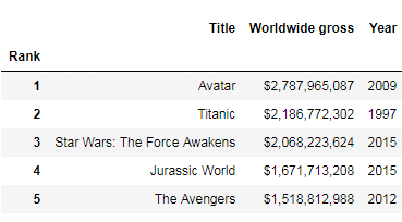
As you can see, passing inplace=True did modify the original DataFrame. Not all methods require the use of the inplace parameter to modify the original DataFrame. For example, the rename(columns) method modifies the original DataFrame without the inplace parameter:
top_movies.rename(columns = {'Year': 'Release Year'}).head()
It’s a good idea to get familiar with the methods that need inplace and the ones that don’t.
The groupby Method
In this section, you’ll learn about using the groupby method to split and aggregate data into groups. You’ll see how the groupby method works by breaking it into parts. The groupby method will be demonstrated in this section with statistical and other methods. You’ll also learn how to do interesting things with the groupby method’s ability to iterate over the group data.
Start by importing the pandas module into your Jupyter notebook, as you did in the previous section:
import pandas as pd
Then read your CSV dataset:
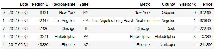
data = pd.read_table('data-zillow.csv', sep=',')
data.head()
Start by asking a question, and see if Pandas’ groupby method can help you get the answer. You want to get the mean Price value of every State:
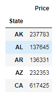
grouped_data = data[['State', 'Price']].groupby('State').mean()
grouped_data.head()
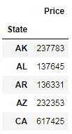
Here, you used the groupby method for aggregating the data by states, and got the mean Price per State. In the background, the groupby method split the data into groups; you then applied the function on the split data, and the result was put together and displayed.
Time to break this code into individual pieces to see what happens under the rug. First, splitting into groups is done as follows:
grouped_data = data[['State', 'Price']].groupby('State')
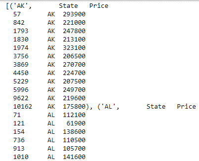
You selected a subset of data that has only State and Price columns. You then called the groupby method on this data, and passed it in the State column, as that is the column you want the data to be grouped by. Then, you stored the data in an object. Print out this data using the list method:
list(grouped_data)
Now, you have the data groups based on date. Next, apply a function on the displayed data, and display the combined result:
grouped_data.mean().head()
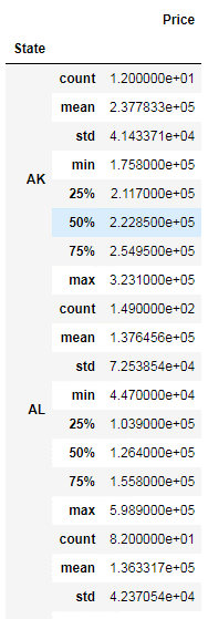
You used the mean method to get the mean of the prices. After the data is split into groups, you can use Pandas methods to get some interesting information on these groups. For example, here, you get descriptive statistical information on each state separately:
grouped_data.describe()
You can also use groupby on multiple columns. For example, here, you’re grouping by the State and RegionName columns, as follows:
grouped_data = data[['State',
                     'RegionName',
                     'Price']].groupby(['State', 'RegionName']).mean()
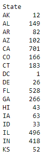
You can also get the number of records per State through the groupby and size methods, as follows:
grouped_data = data.groupby(['State']).size()
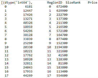
In all the code demonstrated in this section so far, the data has been grouped by rows. However, you can also group by columns. In the following example, this is done by passing the axis parameter set to 1:
grouped_data = data.groupby(data.dtypes, axis=1)
list(grouped_data)
You can also iterate over the split groups, and do interesting things with them, as follows:
for state, grouped_data in data.groupby('State'):
    print(state, 'n', grouped_data)
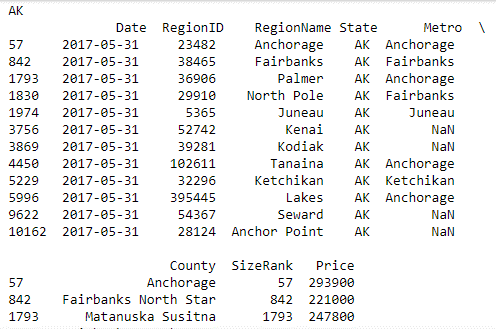 Here, you iterate over the group data by State and publish the result with State as the heading, followed by a table of all the records from that State.
- Learn more by reading the post Descriptive statistics using Python.
Handling Missing Values in Pandas
In this section, you’ll see how to use various pandas techniques to handle the missing data in your datasets. You’ll learn how to find out how much data is missing, and from which columns. You’ll see how to drop the rows or columns where a lot of records are missing data. You’ll also learn how, instead of dropping data, you can fill in the missing records with zeros or the mean of the remaining values.
Start by importing the pandas module into your Jupyter notebook:
import pandas as pd
Then read in your CSV dataset:
data = pd.read_csv('data-titanic.csv')
data.head()
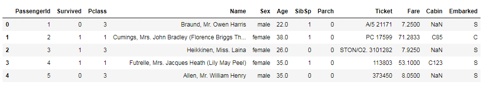 This dataset is the Titanic’s passenger survival dataset, available for download from Kaggle at https://www.kaggle.com/c/titanic/data.
Now take a look at how many records are missing first. To do this, you first need to find out the total number of records in the dataset. You can do this by calling the shape property on the DataFrame:
data.shape
 You can see that the total number of records is 891 and that the total number of columns is 12.
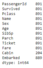
Then it’s time to find out the number of records in each column. You can do this by calling the count method on the DataFrame:
data.count()
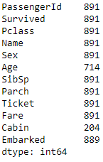 The difference between the total records and the count per column represents the number of records missing from that column. Out of the 12 columns, you have 3 columns where values are missing. For example, Age has only 714 values out of a total of 891 rows; Cabin has values for only 204 records; and Embarked has values for 889 records.
There are different ways of handling these missing values. One of the ways is to drop any row where a value is missing, even from a single column, as follows:
data_missing_dropped = data.dropna()
data_missing_dropped.shape
When you run this method, you assign the results back into a new DataFrame. This leaves you with just 183 records out of a total of 891. However, this may lead to losing a lot of the data, and may not be acceptable.
Another method is to drop only those rows where all the values are missing. Here’s an example:
data_all_missing_dropped = data.dropna(how="all")
data_all_missing_dropped.shape
You do this by setting the how parameter for the dropna method to all.
Instead of dropping rows, another method is to fill in the missing values with some data. You can fill in the missing values with 0, for example, as in the following screenshot:
data_filled_zeros = data.fillna(0)
data_filled_zeros.count()
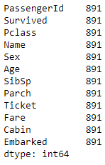 Here, you’ve used the fillna method and passed the numeric value of 0 to the column you want to fill the data in. You can see that you have now filled all the missing values with 0, which is why the count for all the columns has gone up to the total number of count of records in the dataset.
Also, instead of filling in missing values with 0, you could fill them with the mean of the remaining existing values. To do so, call the fillna method on the column where you want to fill the values in and pass the mean of the column as the parameter:
data_filled_in_mean = data.copy()
data_filled_in_mean.Age.fillna(data.Age.mean(), inplace=True)
data_filled_in_mean.count()
 For example, here, you filled in the missing value of Age with the mean of the existing values.
If you found this article interesting and want to learn more about data analysis, you can explore Mastering Exploratory Analysis with pandas, an end-to-end guide to exploratory analysis for budding data scientists. Filled with several hands-on examples, the book is the ideal resource for data scientists as well as Python developers looking to step into the world of exploratory analysis.
The post Data Manipulation with Pandas: A Brief Tutorial appeared first on Erik Marsja.