Introduction
One of my favorite things about Python is that users get the benefit of observing the R community and then emulating the best parts of it. I’m a big believer that a language is only as helpful as its libraries and tools.
This post is about pandasql, a Python package we (Yhat) wrote that emulates the R package sqldf. It’s a small but mighty library comprised of just 358 lines of code. The idea of pandasql is to make Python speak SQL. For those of you who come from a SQL-first background or still “think in SQL”, pandasql is a nice way to take advantage of the strengths of both languages.
In this introduction, we’ll show you to get up and running with pandasql inside of Rodeo, the integrated development environment (IDE) we built for data exploration and analysis. Rodeo is an open source and completely free tool. If you’re an R user, its a comparable tool with a similar feel to RStudio. As of today, Rodeo can only run Python code, but last week we added syntax highlighting of a bunch of other languages to the editor view (mardown, JSON, julia, SQL, markdown). As you may have read or guessed, we’ve got big plans for Rodeo, including adding SQL support so that you can run your SQL queries right inside of Rodeo, even without our handy little pandasql. More on that in the next week or two!
Downloading Rodeo
Start by downloading Rodeo for Mac, Windows or Linux from the Rodeo page on the Yhat website.
ps If you download Rodeo and encounter a problem or simply have a question, we monitor our discourse forum 24/7 (okay, almost).
A bit of background, if you’re curious
Behind the scenes, pandasql uses the pandas.io.sql module to transfer data between DataFrame and SQLite databases. Operations are performed in SQL, the results returned, and the database is then torn down. The library makes heavy use of pandas write_frame and frame_query, two functions which let you read and write to/from pandas and (most) any SQL database.
Install pandasql
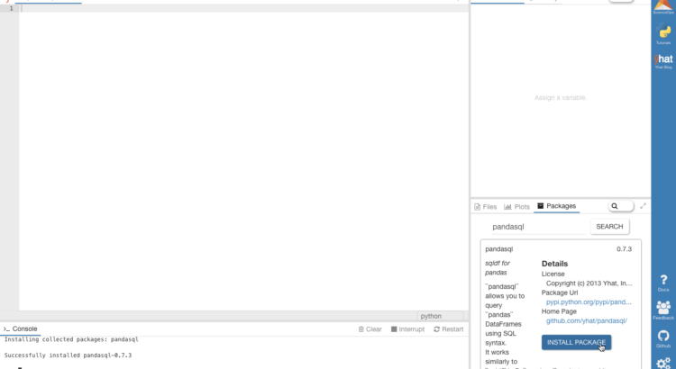
Install pandasql using the package manager pane in Rodeo. Simply search for pandasql and click Install Package.
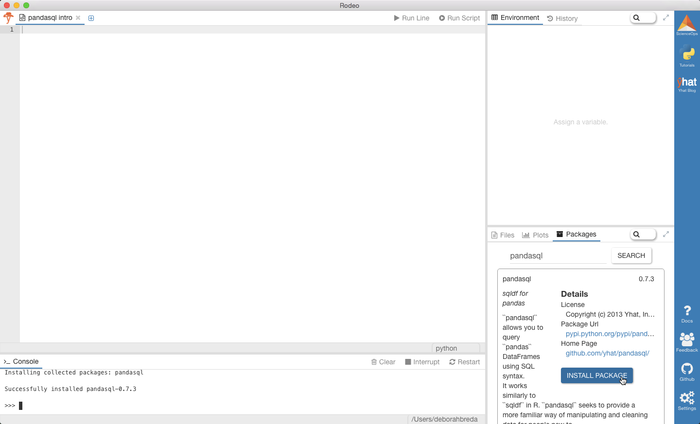
You can also run ! pip install pandasql from the text editor if you prefer to install that way.
Check out the datasets
pandasql has two built-in datasets which we’ll use for the examples below.
meat: Dataset from the U.S. Dept. of Agriculture containing metrics on livestock, dairy, and poultry outlook and productionbirths: Dataset from the United Nations Statistics Division containing demographic statistics on live births by month
Run the following code to check out the data sets.
#Checking out meat and birth data
from pandasql import sqldf
from pandasql import load_meat, load_births
meat = load_meat()
births = load_births()
#You can inspect the dataframes directly if you're using Rodeo
#These print statements are here just in case you want to check out your data in the editor, too
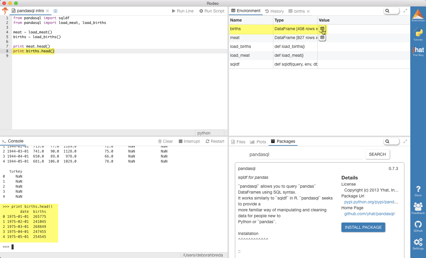
print meat.head()
print births.head()
Inside Rodeo, you really don’t even need the print.variable.head() statements, since you can actually just examine the dataframes directly.
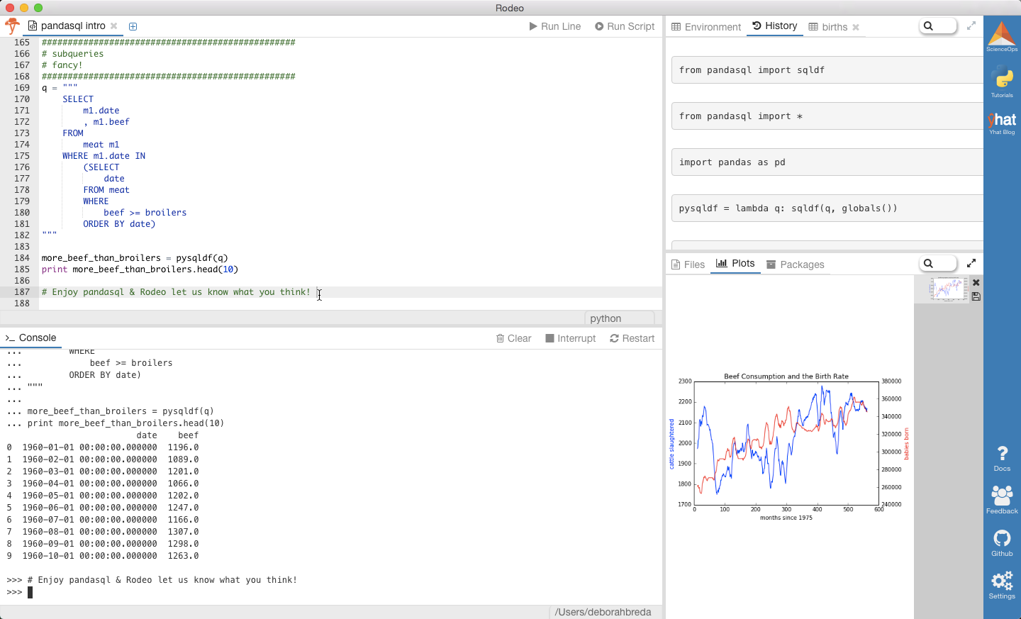
An odd graph
# Let's make a graph to visualize the data
# Bet you haven't had a title quite like this before
import matplotlib.pyplot as plt
from pandasql import *
import pandas as pd
pysqldf = lambda q: sqldf(q, globals())
q = """
SELECT
m.date
, m.beef
, b.births
FROM
meat m
LEFT JOIN
births b
ON m.date = b.date
WHERE
m.date > '1974-12-31';
"""
meat = load_meat()
births = load_births()
df = pysqldf(q)
df.births = df.births.fillna(method='backfill')
fig = plt.figure()
ax1 = fig.add_subplot(111)
ax1.plot(pd.rolling_mean(df['beef'], 12), color='b')
ax1.set_xlabel('months since 1975')
ax1.set_ylabel('cattle slaughtered', color='b')
ax2 = ax1.twinx()
ax2.plot(pd.rolling_mean(df['births'], 12), color='r')
ax2.set_ylabel('babies born', color='r')
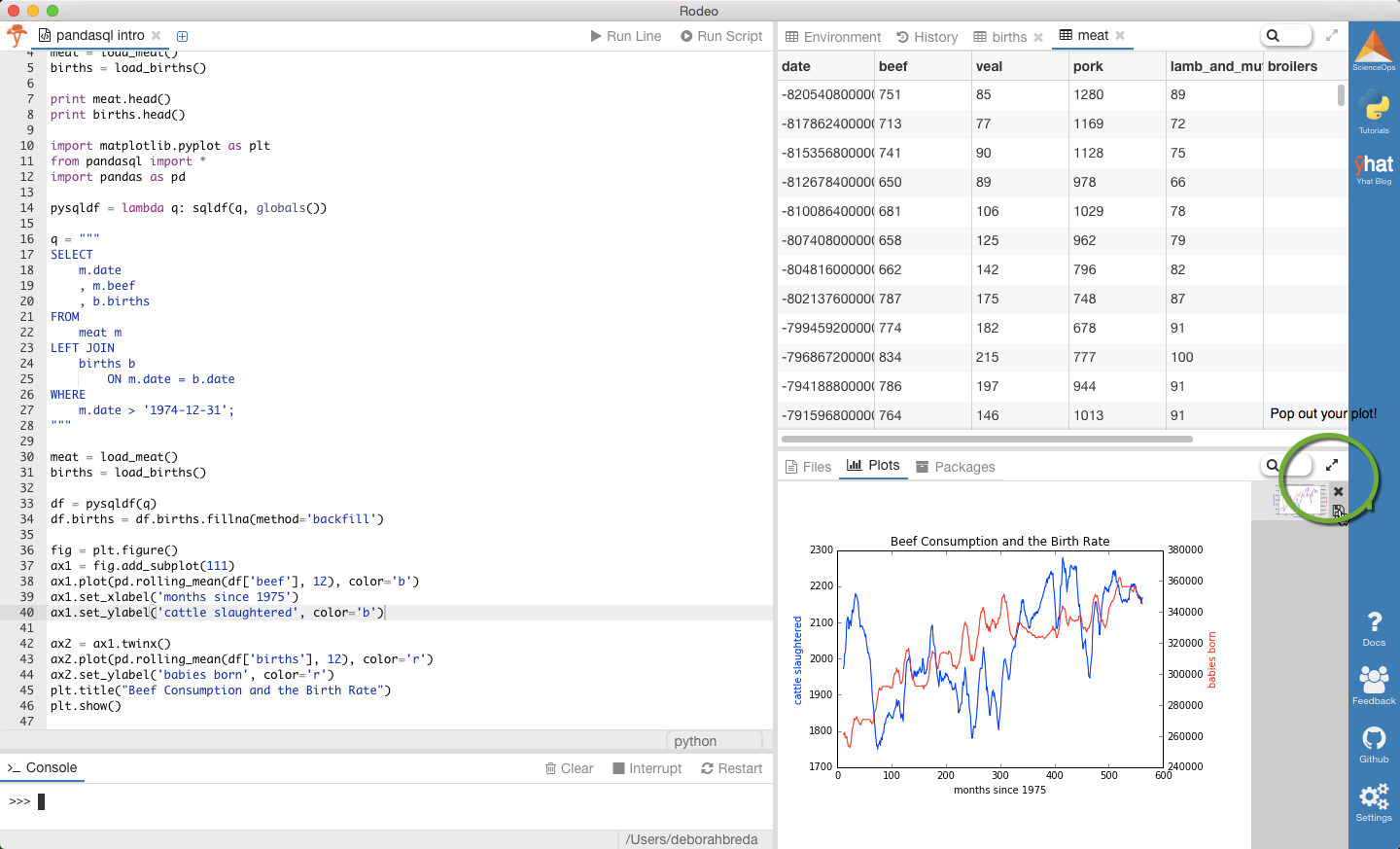
plt.title("Beef Consumption and the Birth Rate")
plt.show()
Notice that the plot appears both in the console and the plot tab (bottom right tab).
Tip: You can “pop out” your plot by clicking the arrows at the top of the pane. This is handy if you’re working on muliple monitors and want to dedicate one just to your data visualzations.
Usage
To keep this post concise and easy to read, we’ve just given the code snippets and a few lines of results for most of the queries below.
If you’re following along in Rodeo, a few tips as you’re getting started:
Run Scriptwill indeed run everything you have written in the text editor- You can highlight a code chunk and run it by clicking
Run Lineor pressing Command + Enter - You can resize the panes (when I’m not making plots I shrink down the bottom right pane)
Basics
Write some SQL and execute it against your pandas DataFrame by substituting DataFrames for tables.
    q = """
        SELECT
            *
        FROM
            meat
        LIMIT 10;"""

    print sqldf(q, locals())

    #                   date  beef  veal  pork  lamb_and_mutton broilers other_chicken turkey
    # 0  1944-01-01 00:00:00   751    85  1280               89     None          None   None
    # 1  1944-02-01 00:00:00   713    77  1169               72     None          None   None
    # 2  1944-03-01 00:00:00   741    90  1128               75     None          None   None
    # 3  1944-04-01 00:00:00   650    89   978               66     None          None   None
pandasql creates a DB, schema and all, loads your data, and runs your SQL.
Aggregation
pandasql supports aggregation. You can use aliased column names or column numbers in your group by clause.
    # births per year
    q = """
        SELECT
            strftime("%Y", date)
            , SUM(births)
        FROM births
        GROUP BY 1
        ORDER BY 1;
                """

    print sqldf(q, locals())

    #    strftime("%Y", date)  SUM(births)
    # 0                  1975      3136965
    # 1                  1976      6304156
    # 2                  1979      3333279
    # 3                  1982      3612258
locals() vs. globals()
pandasql needs to have access to other variables in your session/environment. You can pass locals() to pandasql when executing a SQL statement, but if you’re running a lot of queries that might be a pain. To avoid passing locals all the time, you can add this helper function to your script to set globals() like so:
    def pysqldf(q):
        return sqldf(q, globals())

    q = """
        SELECT
            *
        FROM
            births
        LIMIT 10;"""

    print pysqldf(q)
    # 0  1975-01-01 00:00:00  265775
    # 1  1975-02-01 00:00:00  241045
    # 2  1975-03-01 00:00:00  268849
joins
You can join dataframes using normal SQL syntax.
    # joining meats + births on date
    q = """
        SELECT
            m.date
            , b.births
            , m.beef
        FROM
            meat m
        INNER JOIN
            births b
                on m.date = b.date
        ORDER BY
            m.date
        LIMIT 100;
        """

    joined = pysqldf(q)
    print joined.head()
    #date  births    beef
    #0  1975-01-01 00:00:00.000000  265775  2106.0
    #1  1975-02-01 00:00:00.000000  241045  1845.0
    #2  1975-03-01 00:00:00.000000  268849  1891.0
WHERE conditions
    Here's a `WHERE` clause.

    q = """
        SELECT
            date
            , beef
            , veal
            , pork
            , lamb_and_mutton
        FROM
            meat
        WHERE
            lamb_and_mutton >= veal
        ORDER BY date DESC
        LIMIT 10;
        """

    print pysqldf(q)
    #                   date    beef  veal    pork  lamb_and_mutton
    # 0  2012-11-01 00:00:00  2206.6  10.1  2078.7             12.4
    # 1  2012-10-01 00:00:00  2343.7  10.3  2210.4             14.2
    # 2  2012-09-01 00:00:00  2016.0   8.8  1911.0             12.5
    # 3  2012-08-01 00:00:00  2367.5  10.1  1997.9             14.2
It’s just SQL
Since pandasql is powered by SQLite3, you can do most anything you can do in SQL. Here are some examples using common SQL features such as subqueries, order by, functions, and unions.
    #################################################
    # SQL FUNCTIONS
    # e.g. `RANDOM()`
    #################################################
    q = """SELECT
        *
        FROM
            meat
        ORDER BY RANDOM()
        LIMIT 10;"""
    print pysqldf(q)
    #                   date  beef  veal  pork  lamb_and_mutton  broilers other_chicken  turkey
    # 0  1967-03-01 00:00:00  1693    65  1136               61     472.0          None    26.5
    # 1  1944-12-01 00:00:00   764   146  1013               91       NaN          None     NaN
    # 2  1969-06-01 00:00:00  1666    50   964               42     573.9          None    85.4
    # 3  1983-03-01 00:00:00  1892    37  1303               36    1106.2          None   182.7

    #################################################
    # UNION ALL
    #################################################
    q = """
            SELECT
                date
                , 'beef' AS meat_type
                , beef AS value
            FROM meat
            UNION ALL
            SELECT
                date
                , 'veal' AS meat_type
                , veal AS value
            FROM meat

            UNION ALL

            SELECT
                date
                , 'pork' AS meat_type
                , pork AS value
            FROM meat
            UNION ALL
            SELECT
                date
                , 'lamb_and_mutton' AS meat_type
                , lamb_and_mutton AS value
            FROM meat
            ORDER BY 1
        """
    print pysqldf(q).head(20)
    #                    date        meat_type  value
    # 0   1944-01-01 00:00:00             beef    751
    # 1   1944-01-01 00:00:00             veal     85
    # 2   1944-01-01 00:00:00             pork   1280
    # 3   1944-01-01 00:00:00  lamb_and_mutton     89


    #################################################
    # subqueries
    # fancy!
    #################################################
    q = """
        SELECT
            m1.date
            , m1.beef
        FROM
            meat m1
        WHERE m1.date IN
            (SELECT
                date
            FROM meat
            WHERE
                beef >= broilers
            ORDER BY date)
    """

    more_beef_than_broilers = pysqldf(q)
    print more_beef_than_broilers.head(10)
    #                   date  beef
    # 0  1960-01-01 00:00:00  1196
    # 1  1960-02-01 00:00:00  1089
    # 2  1960-03-01 00:00:00  1201
    # 3  1960-04-01 00:00:00  1066
Final thoughts
pandas is an incredible tool for data analysis in large part, we think, because it is extremely digestible, succinct, and expressive. Ultimately, there are tons of reasons to learn the nuances of merge, join, concatenate, melt and other native pandas features for slicing and dicing data. Check out the docs for some examples.
Our hope is that pandasql will be a helpful learning tool for folks new to Python and pandas. In my own personal experience learning R, sqldf was a familiar interface helping me become highly productive with a new tool as quickly as possible.
We hope you’ll check out pandasql and Rodeo; if you do, please let us know what you think!