So far the petersburg project has been primarily focused on static modeling of complex decisions with uncertainty. The longer-term goal is for it to to be a fully-feature toolbox for supporting such decisions. In that context, I’ve posted previously about:
- Decision strategies
- How the petersburg framework works
- How petersburg differs from bayesian networks
And more. In this post, we will begin to explore how we can use the petersburg framework in a forward looking sense, for estimation.
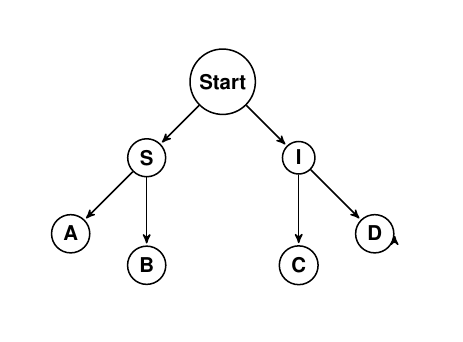
Petersburg represents complex decisions as directed acyclic graphs, which allows the user to enforce a known structure to the problem. In this post, we will use a medical diagnosis as the example. Take the petersburg DAG (pDAG) below:

Upon entrance into our hypothetical ER, the patient can be either sick or injured. We know of two sickness and two injuries. So our hierarchy has just two layers (1 and 2). We could encode this numerically as:
| {S|I} | {A|B|C|D} |
|---|---|
| 1 | 1 |
| 1 | 2 |
| 2 | 3 |
| 2 | 4 |
In the absolute simplest case, we could have a person sit at the door of our ER and record what people had on their way out. A new row indicating what the diagnosis was could be added in, and gradually we would build a frequentist dataset from which we could draw some conclusions.
In practice, that means that we want to stream data into an adjacency matrix of the graph. We can give each node an index, and represent an observed traversal by incrementing the value in entry (from_node, to_node). So the above data would look like:
| 0 | S | I | A | B | C | D | |
|---|---|---|---|---|---|---|---|
| 0 | 0 | 0 | 0 | 0 | 0 | 0 | 0 |
| S | 2 | 0 | 0 | 0 | 0 | 0 | 0 |
| I | 2 | 0 | 0 | 0 | 0 | 0 | 0 |
| A | 0 | 1 | 0 | 0 | 0 | 0 | 0 |
| B | 0 | 1 | 0 | 0 | 0 | 0 | 0 |
| C | 0 | 0 | 1 | 0 | 0 | 0 | 0 |
| D | 0 | 0 | 1 | 0 | 0 | 0 | 0 |
As people come through the ER, we can just update this adjacency matrix, and use petersburg’s new from_adj_matrix() to generate a petersburg graph object whenever we want to run simulations.
Let’s say that as we continue on, 100 people walk in with sickness A. Our updated matrix looks like:
| 0 | S | I | A | B | C | D | |
|---|---|---|---|---|---|---|---|
| 0 | 0 | 0 | 0 | 0 | 0 | 0 | 0 |
| S | 102 | 0 | 0 | 0 | 0 | 0 | 0 |
| I | 2 | 0 | 0 | 0 | 0 | 0 | 0 |
| A | 0 | 101 | 0 | 0 | 0 | 0 | 0 |
| B | 0 | 1 | 0 | 0 | 0 | 0 | 0 |
| C | 0 | 0 | 1 | 0 | 0 | 0 | 0 |
| D | 0 | 0 | 1 | 0 | 0 | 0 | 0 |
And a simulation of the pDAG will show that A is the most likely outcome.
This is, of course, a very simplistic case. The interesting part here is that the estimation problem gets implicitly broken down into many smaller conditional probability problems, so we may not be able to well predict P(A|S), but if we have a good model for P(S), then we can use the frequency estimates to augment that good prediction of P(S) with actionable estimates at the lower level.
This first step has been implemented in the python library for petersburg as a scikit-learn style estimator, which supports partial fit for streaming in data as incremental updates. Using randomly generated data, we have an example here:
import numpy as np
import random
import json
from petersburg import FrequencyEstimator

zero_count = 11
one_count = 32
two_count = 55
three_count = 50
four_count = 21
total = zero_count + one_count + two_count + three_count + four_count

# generate some data
y = np.array([[
    random.choice([0, 1, 2]),
    random.choice([0, 1, 1, 1, 2]),
    random.choice([0, 1, 2, 2, 2, 2]),
    random.choice(
        [0 for _ in range(zero_count)] +
        [1 for _ in range(one_count)] +
        [2 for _ in range(two_count)] +
        [3 for _ in range(three_count)] +
        [4 for _ in range(four_count)]
    )
] for _ in range(10000)])

# train a frequency estimator
clf = FrequencyEstimator(verbose=True)
clf.fit(None, y)
freq_matrix = clf._frequency_matrix
y_hat = clf.predict(np.zeros((10000, 10)))

# print out what we've learned from it
print('nCategory Labels')
labels = clf._cateogry_labels
print(labels)

print('nUnique Predicted Outcomes')
outcomes = sorted([str(labels[int(x)]) for x in set(y_hat.reshape(-1, ).tolist())])
print(outcomes)

print('nHistogram')
histogram = dict(zip(outcomes, [float(x) for x in np.histogram(y_hat, bins=[8.5, 9.5, 10.5, 11.5, 12.5, 13.5])[0]]))
print(json.dumps(histogram, sort_keys=True, indent=4))
Which will output:
Category Labels
{0: (0, 0), 1: (0, 1), 2: (0, 2), 3: (1, 0), 4: (1, 1), 5: (1, 2), 6: (2, 0), 7: (2, 1), 8: (2, 2), 9: (3, 0), 10: (3, 1), 11: (3, 2), 12: (3, 3), 13: (3, 4)}

Unique Predicted Outcomes
['(3, 0)', '(3, 1)', '(3, 2)', '(3, 3)', '(3, 4)']

Histogram
{
    "(3, 0)": 706.0,
    "(3, 1)": 1898.0,
    "(3, 2)": 3211.0,
    "(3, 3)": 3019.0,
    "(3, 4)": 1166.0
}
As development on the library continues we are targeting:
- Petersburg graph object as an accessible attribute of the estimator
- Selective inclusion of weak classifiers for estimation of conditional probabilities (where CV scores support their use, otherwise fall back to frequency)
- Different outputs (currently output is a single simulated outcome)
All of this is on github, and development is slated to continue onward, so try out the library or contact me if you’d like to help develop it further.
https://github.com/wdm0006/petersburg
The post Simple estimation of hierarchical events with petersburg appeared first on Will’s Noise.