For this post, I want to describe a text analytics and visualization technique using a basic keyword extraction mechanism using nothing but a word counter to find the top 3 keywords from a corpus of articles that I’ve created from my blog at http://ericbrown.com. To create this corpus, I downloaded all of my blog posts (~1400 of them) and grabbed the text of each post. Then, I tokenize the post using nltk and various stemming / lemmatization techniques, count the keywords and take the top 3 keywords. I then aggregate all keywords from all posts to create a visualization using Gephi.
I’ve uploaded a jupyter notebook with the full code-set for you to replicate this work. You can also get a subset of my blog articles in a csv file here. You’ll need beautifulsoup and nltk installed. You can install them with:
pip install bs4 nltk
To get started, let’s load our libraries:
import pandas as pd
import numpy as np

from nltk.tokenize import word_tokenize, sent_tokenize
from nltk.corpus import stopwords
from nltk.stem import WordNetLemmatizer, PorterStemmer
from string import punctuation
from collections import Counter

from collections import OrderedDict
import re
import warnings
warnings.filterwarnings("ignore", category=DeprecationWarning)

from HTMLParser import HTMLParser
from bs4 import BeautifulSoup
I’m loading warnings here because there’s a warning about BeautifulSoup that we can ignore.
Now, let’s set up some things we’ll need for this work.
First, let’s set up our stop words, stemmers and lemmatizers.
porter = PorterStemmer()
wnl = WordNetLemmatizer()
stop = stopwords.words('english')
stop.append("new")
stop.append("like")
stop.append("u")
stop.append("it'")
stop.append("'s")
stop.append("n't")
stop.append('mr.')
stop = set(stop)
Now, let’s set up some functions we’ll need.
The tokenizer function is taken from here. If you want to see some cool topic modeling, jump over and read How to mine newsfeed data and extract interactive insights in Python…its a really good article that gets into topic modeling and clustering…which is something I’ll hit on here as well in a future post.
# From http://ahmedbesbes.com/how-to-mine-newsfeed-data-and-extract-interactive-insights-in-python.html

def tokenizer(text):

    tokens_ = [word_tokenize(sent) for sent in sent_tokenize(text)]

    tokens = []
    for token_by_sent in tokens_:
        tokens += token_by_sent

    tokens = list(filter(lambda t: t.lower() not in stop, tokens))
    tokens = list(filter(lambda t: t not in punctuation, tokens))
    tokens = list(filter(lambda t: t not in [u"'s", u"n't", u"...", u"''", u'``', u'u2014', u'u2026', u'u2013'], tokens))

    filtered_tokens = []
    for token in tokens:
        token = wnl.lemmatize(token)
        if re.search('[a-zA-Z]', token):
            filtered_tokens.append(token)

    filtered_tokens = list(map(lambda token: token.lower(), filtered_tokens))

    return filtered_tokens
Next, I had some html in my articles, so i wanted to strip it from my text before doing anything else with it…here’s a class to do that using bs4. I found this code on Stackoverflow.
class MLStripper(HTMLParser):
    def __init__(self):
        self.reset()
        self.fed = []
    def handle_data(self, d):
        self.fed.append(d)
    def get_data(self):
        return ''.join(self.fed)

def strip_tags(html):
    s = MLStripper()
    s.feed(html)
    return s.get_data()
OK – now to the fun stuff. To get our keywords, we need only 2 lines of code. This function does a count and returns said count of keywords for us.
def get_keywords(tokens, num):
    return Counter(tokens).most_common(num)
Finally, I created a function to take a pandas dataframe filled with urls/pubdate/author/text and then create my keywords from that. This function iterates over a pandas dataframe (each row is an article from my blog), tokenizes the ‘text’ from and returns a pandas dataframe with keywords, the title of the article and the publication data of the article.
def build_article_df(urls):
    articles = []
    for index, row in urls.iterrows():
        try:
            data=row['text'].strip().replace("'", "")
            data = strip_tags(data)
            soup = BeautifulSoup(data)
            data = soup.get_text()
            data = data.encode('ascii', 'ignore').decode('ascii')
            document = tokenizer(data)
            top_5 = get_keywords(document, 5)

            unzipped = zip(*top_5)
            kw= list(unzipped[0])
            kw=",".join(str(x) for x in kw)
            articles.append((kw, row['title'], row['pubdate']))
        except Exception as e:
            print e
            #print data
            #break
            pass
        #break
    article_df = pd.DataFrame(articles, columns=['keywords', 'title', 'pubdate'])
    return article_df
Time to load the data and start analyzing. This bit of code loads in my blog articles (found here) and then grabs only the interesting columns from the data, renames them and prepares them for tokenization. Most of this can be done in one line when reading in the csv file, but I already had this written for another project and just it as is.
df = pd.read_csv('../examples/tocsv.csv')
data = []
for index, row in df.iterrows():
data.append((row['Title'], row['Permalink'], row['Date'], row['Content']))
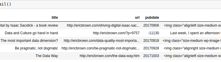
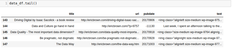
data_df = pd.DataFrame(data, columns=['title' ,'url', 'pubdate', 'text' ])
Taking the tail() of the dataframe gets us:
Now, we can tokenize and do our word-count by calling our build_article_df function.
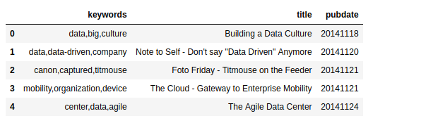
article_df = build_article_df(data_df)
This gives us a new dataframe with the top 3 keywords for each article (along with the pubdate and title of the article).
This is quite cool by itself. We’ve generated keywords for each article automatically using a simple counter. Not terribly sophisticated but it works and works well. There are many other ways to do this, but for now we’ll stick with this one. Beyond just having the keywords, it might be interesting to see how these keywords are ‘connected’ with each other and with other keywords. For example, how many times does ‘data’ shows up in other articles?
There are multiple ways to answer this question, but one way is by visualizing the keywords in a topology / network map to see the connections between keywords. we need to do a ‘count’ of our keywords and then build a co-occurrence matrix. This matrix is what we can then import into Gephi to visualize. We could draw the network map using networkx, but it tends to be tough to get something useful from that without a lot of work…using Gephi is much more user friendly.
We have our keywords and need a co-occurance matrix. To get there, we need to take a few steps to get our keywords broken out individually.
keywords_array=[]
for index, row in article_df.iterrows():
    keywords=row['keywords'].split(',')
    for kw in keywords:
        keywords_array.append((kw.strip(' '), row['keywords']))
kw_df = pd.DataFrame(keywords_array).rename(columns={0:'keyword', 1:'keywords'})
We now have a keyword dataframe kw_df that holds two columns: keyword and keywords with keyword
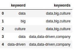
This doesn’t really make a lot of sense yet, but we need both columns to build a co-occurance matrix. We do by iterative over each document keyword list (the keywords column) and seeing if the keyword is included. If so, we added to our occurance matrix and then build our co-occurance matrix.
document = kw_df.keywords.tolist()
names = kw_df.keyword.tolist()

document_array = []
for item in document:
    items = item.split(',')
    document_array.append((items))

occurrences = OrderedDict((name, OrderedDict((name, 0) for name in names)) for name in names)

# Find the co-occurrences:
for l in document_array:
    for i in range(len(l)):
        for item in l[:i] + l[i + 1:]:
            occurrences[l[i]][item] += 1

co_occur = pd.DataFrame.from_dict(occurrences )
Now, we have a co-occurance matrix in the co_occur dataframe, which can be imported into Gephi to view a map of nodes and edges. Save the co_occur dataframe as a CSV file for use in Gephi (you can download a copy of the matrix here).
co_occur.to_csv('out/ericbrown_co-occurancy_matrix.csv')
Over to Gephi
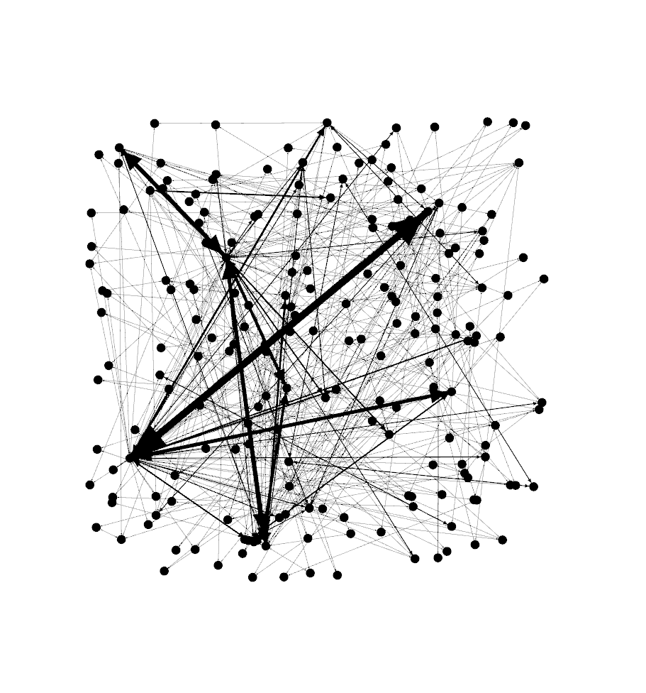
Now, its time to play around in Gephi. I’m a novice in the tool so can’t really give you much in the way of a tutorial, but I can tell you the steps you need to take to build a network map. First, import your co-occuance matrix csv file using File -> Import Spreadsheet and just leave everything at the default. Then, in the ‘overview’ tab, you should see a bunch of nodes and connections like the image below.
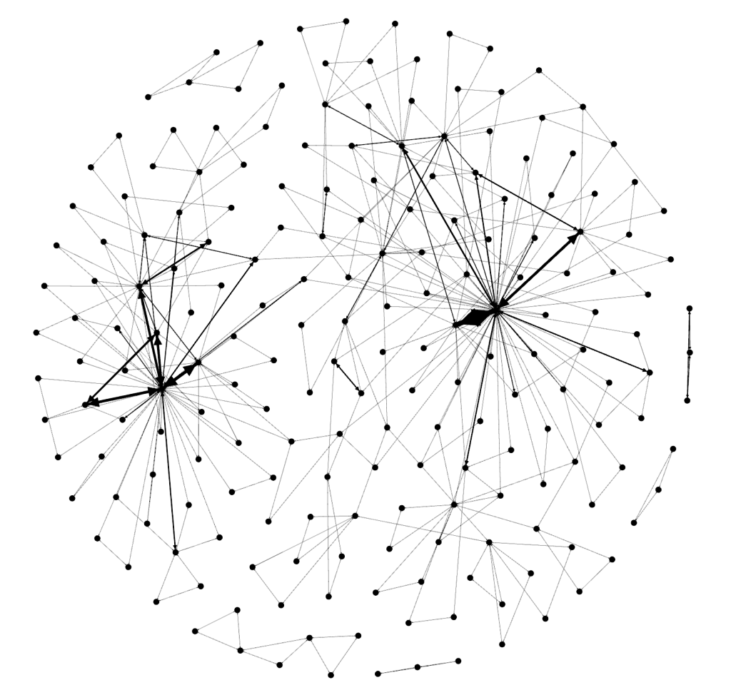
Next, move down to the ‘layout’ section and select the Fruchterman Reingold layout and push ‘run’ to get the map to redraw. At some point, you’ll need to press ‘stop’ after the nodes settle down on the screen. You should see something like the below.
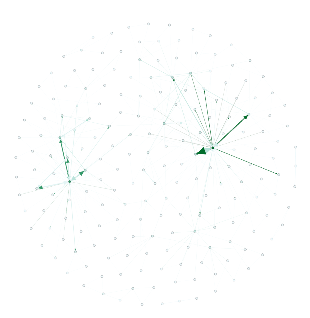
Cool, huh? Now…let’s get some color into this graph. In the ‘appearance’ section, select ‘nodes’ and then ‘ranking’. Select “Degree’ and hit ‘apply’. You should see the network graph change and now have some color associated with it. You can play around with the colors if you want but the default color scheme should look something like the following:
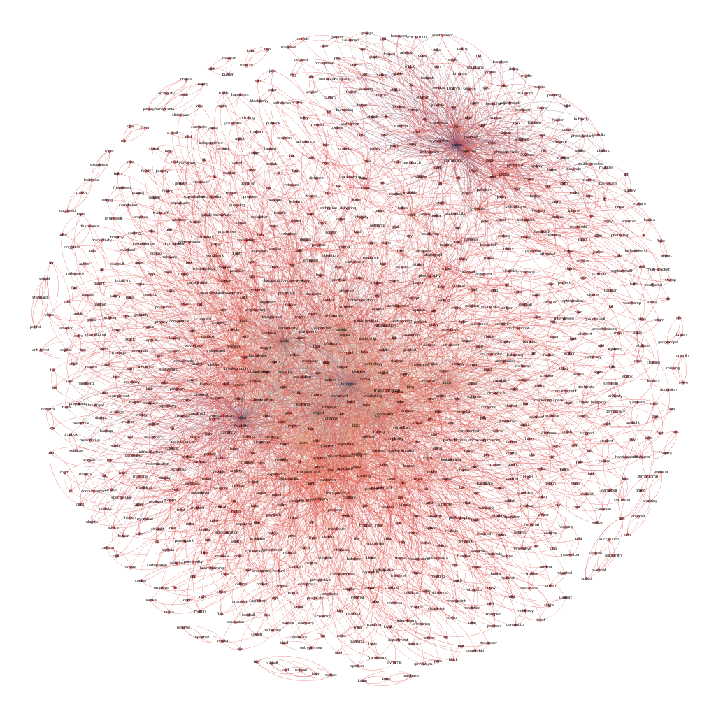
Still not quite interesting though. Where’s the text/keywords? Well…you need to swtich over to the ‘overview’ tab to see that. You should see something like the following (after selecting ‘Default Curved’ in the drop-down.
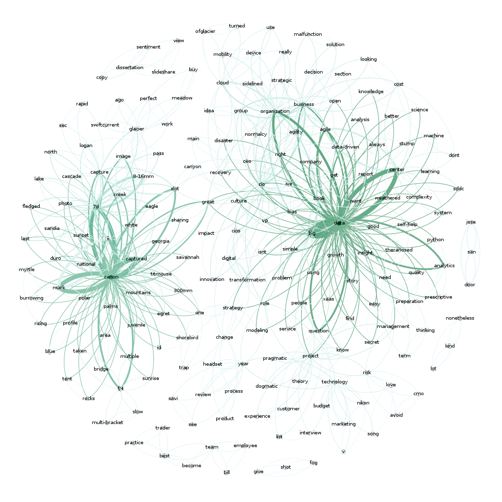
Now that’s pretty cool. You can see two very distinct areas of interest here. “Data’ and “Canon”…which makes sense since I write a lot about data and share a lot of my photography (taken with a Canon camera).
Here’s a full map of all 1400 of my articles if you are interested. Again, there are two main clusters around photography and data but there’s also another large cluster around ‘business’, ‘people’ and ‘cio’, which fits with what most of my writing has been about over the years.
There are a number of other ways to visualize text analytics. I’m planning a few additional posts to talk about some of the more interesting approaches that I’ve used and run across recently. Stay tuned.
If you want to learn more about Text analytics, check out these books:
Natural Language Processing with Python: Analyzing Text with the Natural Language Toolkit
The post Text Analytics and Visualization appeared first on Python Data.