Probabilistic Programming in Python

Learn about probabilistic programming in this guest post by Osvaldo Martin, a researcher at The National Scientific and Technical Research Council (CONICET).

Bayesian Inference

Bayesian statistics is conceptually very simple; we have the knowns and the unknowns; we use Bayes’ theorem to condition the latter on the former. If we are lucky, this process will reduce the uncertainty about the unknowns.

Generally, we refer to the knowns as data and treat it like a constant, and the unknowns as parameters and treat them as probability distributions. In more formal terms, we assign probability distributions to unknown quantities. Then, we use Bayes’ theorem to transform the prior probability distribution

 

into a posterior distribution:

 

Although conceptually simple, fully probabilistic models often lead to analytically intractable expressions. For many years, this was a real problem and was probably one of the main issues that hindered the wide adoption of Bayesian methods.

The arrival of the computational era and the development of numerical methods that, at least in principle, can be used to solve any inference problem, has dramatically transformed the Bayesian data analysis practice.

Probabilistic Programming: the Inference-Button

We can think of these numerical methods as universal inference engines, or as Thomas Wiecki, the core developer of PyMC3, likes to call it, the inference-button. The possibility of automating the inference process has led to the development of probabilistic programming languages (PPL), which allow for a clear separation between model creation and inference.

In the PPL framework, users specify a full probabilistic model by writing a few lines of code, and then inference follows automatically. It is expected that probabilistic programming will have a major impact on data science and other disciplines by enabling practitioners to build complex probabilistic models in a less time-consuming and less error-prone way.

I think one good analogy for the impact that programming languages can have on scientific computing is the introduction of the Fortran programming language more than six decades ago. While Fortran has lost its shine nowadays, at one time, it was considered to be very revolutionary.

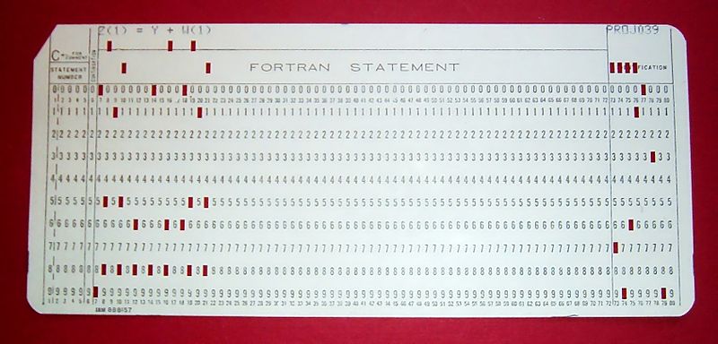
For the first time, scientists moved away from computational details and began focusing on building numerical methods, models, and simulations in a more natural way. In a similar fashion, we now have PPL, which hides details on how probabilities are manipulated and how the inference is performed from users, allowing users to focus on model specification and the analysis of the results.

In this article, you will learn how to use PyMC3 to define and solve models. We will treat the inference-button as a black box that gives us proper samples from the posterior distribution. The methods we will be using are stochastic, and so the samples will vary every time we run them.

However, if the inference process works as expected, the samples will be representative of the posterior distribution and thus we will obtain the same conclusion from any of those samples.

PyMC3 primer

PyMC3 is a Python library for probabilistic programming. The latest version at the moment of writing is 3.6. PyMC3 provides a very simple and intuitive syntax that is easy to read and close to the syntax used in statistical literature to describe probabilistic models. PyMC3’s base code is written using Python, and the computationally demanding parts are written using NumPy and Theano.

What is Theano?

Theano is a Python library that was originally developed for deep learning and allows us to define, optimize, and evaluate mathematical expressions involving multidimensional arrays efficiently. The main reason PyMC3 uses Theano is because some of the sampling methods, such as NUTS, need gradients to be computed, and Theano knows how to compute gradients using what is known as automatic differentiation.

Also, Theano compiles Python code to C code, and hence PyMC3 is really fast. This is all the information about Theano we need to have to use PyMC3. If you still want to learn more about it, start reading the official Theano tutorial at http://deeplearning.net/software/theano/tutorial/index.html#tutorial.

Flipping coins the PyMC3 way

We’ll be generating some fictional data, so you can assume that we know the true value of

, called theta_real, in the following code. Of course, for a real dataset, we will not have this knowledge:

np.random.seed(123)

trials = 4

theta_real = 0.35 # unknown value in a real experiment

data = stats.bernoulli.rvs(p=theta_real, size=trials)

Model specification

Now that we have the data, we need to specify the model. This is done by specifying the likelihood and the prior using probability distributions. For the likelihood, we will use the binomial distribution with

 and

, and for the prior, a beta distribution with the parameters:

A beta distribution with such parameters is equivalent to a uniform distribution in the interval [0, 1]. We can write the model using the following mathematical notation:

 

This statistical model has an almost one-to-one translation to PyMC3:

with pm.Model() as our_first_model:

    θ = pm.Beta('θ', alpha=1., beta=1.)

    y = pm.Bernoulli('y', p=θ, observed=data)

    trace = pm.sample(1000, random_seed=123)

The first line of the code creates a container for our model. Everything inside the with-block will be automatically added to our_first_model. You can think of this as syntactic sugar to ease model specification as we do not need to manually assign variables to the model. The second line specifies the prior. As you can see, the syntax follows the mathematical notation closely.

The third line specifies the likelihood. The syntax is almost the same as for the prior, except that we pass the data using the observed argument. In this way, we can tell PyMC3 that we want to condition for the unknown on the knowns (data). The observed values can be passed as a Python list, a tuple, a NumPy array, or a pandas DataFrame.

Now, we are finished with the model’s specification! Pretty neat, right?

Pushing the inference button

The last line is the inference button. We are asking for 1,000 samples from the posterior and will store them in the trace object. Behind this innocent line, PyMC3 has hundreds of oompa loompas, singing and baking a delicious Bayesian inference just for you! Well, not exactly, but PyMC3 is automating a lot of tasks. If you run the code, you will get a message like this:

Auto-assigning NUTS sampler... 
Initializing NUTS using jitter+adapt_diag... 
Multiprocess sampling (2 chains in 2 jobs) 
NUTS: [θ] 100%|██████████| 3000/3000 [00:00<00:00, 3695.42it/s]

The first and second lines tell us that PyMC3 has automatically assigned the NUTS sampler (one inference engine that works very well for continuous variables), and has used a method to initialize that sampler. The third line says that PyMC3 will run two chains in parallel, so we can get two independent samples from the posterior for the price of one.

The exact number of chains is computed taking into account the number of processors in your machine; you can change it using the chains argument for the sample function. The next line is telling us which variables are being sampled by which sampler.

For this particular case, this line is not adding any new information because NUTS is used to sample the only variable we have θ. However, this is not always the case as PyMC3 can assign different samplers to different variables. This is done automatically by PyMC3 based on the properties of the variables, which ensures that the best possible sampler is used for each variable. Users can manually assign samplers using the step argument of the sample function.

Finally, the last line is a progress bar, with several related metrics indicating how fast the sampler is working, including the number of iterations per second. If you run the code, you will see the progress-bar get updated really fast. Here, we are seeing the last stage when the sampler has finished its work.

The numbers are 3000/3000, where the first number is the running sampler number (this starts at 1), and the last is the total number of samples. You will notice that we have asked for 1,000 samples, but PyMC3 is computing 3,000 samples. We have 500 samples per chain to auto-tune the sampling algorithm (NUTS, in this example).

This sample will be discarded by default. We also have 1,000 productive draws per-chain, thus a total of 3,000 samples are generated. The tuning phase helps PyMC3 provide a reliable sample from the posterior. We can change the number of tuning steps with the tune argument of the sample function.

Summarizing the posterior

Generally, the first task we will perform after sampling from the posterior is check what the results look like. The plot_trace function from ArviZ is ideally suited to this task:

az.plot_trace(trace)

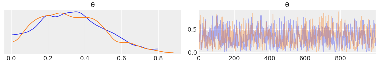
By using az.plot_trace, we get two subplots for each unobserved variable. The only unobserved variable in our model is

Notice that y is an observed variable representing the data; we do not need to sample that because we already know those values. Thus, in the above figure, we have two subplots. On the left, we have a Kernel Density Estimation (KDE) plot; this is like the smooth version of the histogram. On the right, we get the individual sampled values at each step during the sampling. From the trace plot, we can visually get the plausible values from the posterior.

If this article piqued your interest in Bayesian Analysis, you can check out Bayesian Analysis with Python – Second Edition by Osvaldo Martinez. A step-by-step guide following a modern, practical, and computational approach, Bayesian Analysis with Python – Second Edition is a must-read for students, data scientists, developers, and researchers alike who want to get started with probabilistic programming.

The post Probabilistic Programming in Python appeared first on Erik Marsja.