
Machine learning is easily one of the biggest buzzwords in tech right now. Over the past three years Google searches for “machine learning” have increased by over 350%. But understanding machine learning can be difficult — you either use pre-built packages that act like ‘black boxes’ where you pass in data and magic comes out the other end, or you have to deal with high level maths and linear algebra.
This tutorial is designed to introduce you to the fundamental concepts of machine learning — you’ll build your very first model from scratch to make predictions, while understanding exactly how your model works.
This tutorial is based on our Dataquest Machine Learning Fundamentals course, which is part of our Data Science Learning Path. The course goes into a lot more detail, and allows you to follow along writing code to learn by doing.
To start though, let’s explore what machine learning actually is.
What is machine learning?
Machine learning is the practice of building systems, known as models, that can be trained using data to find patterns which can then be used to make predictions on new data.
An important distinction is that a machine learning model is not a rules-based system, where a series of ‘if/then’ statements are used to make predictions (eg ‘If a students misses more than 50% of classes then automatically fail them’). Rather, it is one where statistical relationships are used to learn about the past instances of what we’re predicting, and then are applied to new data.
Let’s look at an example. Say you are selling your house, and you are trying to work out what price to ask for. You can look at other houses that have recently sold in your area, and find those that are most common to yours. Each house you look at is known as an observation. When you’re trying to find similar houses, you might look at the size of the house, how many bedrooms and bathrooms they have, etc. Each of these attributes that you look at are called features.

Similar Houses can help you decide on the price to sell your house for
Once you have found a number of similar houses, you could then look at the price that they sold for, and take an average of that for your house listing.
In this example, the ‘model’ you built was trained on data from other houses in your area — or past observations — and then used to make a recommendation for the price of your house, which is new data the model has not previously seen.
The value you are predicting, the price, is known as the target variable.
The model we’re going to build in this tutorial is similar to the strategy we outlined above. We’re going to be making recommendations for the price that you should list your apartment for on Airbnb by building a simple model using Python.
This post presumes you are familiar with Python’s pandas library — if you need to brush up on pandas, we recommend our two-part pandas tutorial blog posts or our interactive Python and Pandas course.
Predicting Airbnb rental prices
Airbnb is a marketplace for short term rentals, allowing you to list part or all of your living space for others to rent. The company itself has grown rapidly from its founding in 2008 to a 30 billion dollar valuation in 2016 and is currently worth more than any hotel chain in the world.
One challenge that Airbnb hosts face is determining the optimal nightly rent price.
In many areas, renters are presented with a good selection of listings and can filter on criteria like price, number of bedrooms, room type, and more. Since Airbnb is a marketplace, the amount a host can charge on a nightly basis is closely linked to the dynamics of the marketplace. Here’s a screenshot of the search experience on Airbnb:
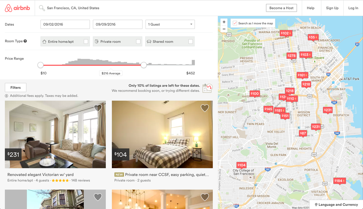
Airbnb Search Results
As hosts, if we try to charge above market price then renters will select more affordable alternatives. If we set our nightly rent price too low, we’ll miss out on potential revenue.
One strategy we could use is to:
- Find a few listings that are similar to ours,
- Average the listed price for the ones most similar to ours,
- Set our listing price to this calculated average price.
We’re going to build a machine learning model to automate this process using a technique called k-nearest neighbors.
First, let’s introduce the data set we’ll be working with.
Our Airbnb Data
While Airbnb doesn’t release any data on the listings in their marketplace, a separate group named Inside Airbnb has extracted data on a sample of the listings for many of the major cities on the website. In this post, we’ll be working with their data set from October 3, 2015 on the listings from Washington, D.C., the capital of the United States. Here’s a direct link to that data set. Each row in the data set is a specific listing that’s available for renting on Airbnb in the Washington, D.C. area
To make the data set less cumbersome to work with, we’ve removed many of the columns in the original data set and renamed the file to dc_airbnb.csv. Here are some of the more important columns:
accommodates: the number of guests the rental can accommodatebedrooms: number of bedrooms included in the rentalbathrooms: number of bathrooms included in the rentalbeds: number of beds included in the rentalprice: nightly price for the rentalminimum_nights: minimum number of nights a guest can stay for the rentalmaximum_nights: maximum number of nights a guest can stay for the rentalnumber_of_reviews: number of reviews that previous guests have left
We’ll read the data set into pandas, print its size and view the first few rows.
import pandas as pd

dc_listings = pd.read_csv('dc_airbnb.csv')
print(dc_listings.shape)

dc_listings.head()
The K-nearest neighbors algorithm
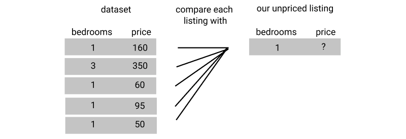
The K-nearest neighbors (knn) algorithm is very similar to the three step process we outlined earlier to compare our listing to similar listings and take the average price. Let’s look at it in some more detail.
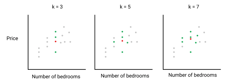
First, we select the number of similar listings, k, that we want to compare with.
Next, we need to calculate how similar each listing is to ours using a similarity metric.
Then we rank each listing using our similarity metric and select the first k listings.
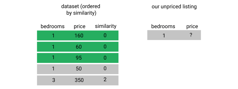
Finally, we calculate the mean price for the k similar listings, and use that as our list price.
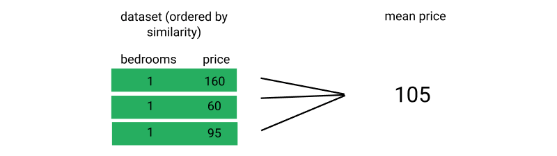
Let’s start by defining what similarity metric we’re going to use. Then, we’ll implement the k-nearest neighbors algorithm and use it to suggest a price for a new, unpriced listing.
For the purposes of this tutorial we’re going to use a fixed k value of 5, but once you become familiar with the workflow around the algorithm you can experiment with this value to see if you get better results with lower or higher k values.
When trying to predict a continuous value, like price, the main similarity metric that’s used is Euclidean distance. Here’s the general formula for Euclidean distance:
where $ q_1 $ to $ q_n $ represent the feature values for one observation and $ p_1 $ to $ p_n $ represent the feature values for the other observation.
Building a simple knn model
Let’s start by simplifying things a little, and looking at just one column. Here’s the formula for just one feature.
The square root and the squared power cancel and the formula simplifies to:
or expressed in words, the absolute value of the difference between the observation and the data point we want to predict for the feature we’re using.
The living space that we want to rent can accommodate three people. Let’s first calculate the distance, using just the accommodates feature, between the first living space in the dataset and our own.
We’ll use the NumPy function np.abs() to easily calculate the absolute value.
import numpy as np

our_acc_value = 3
first_living_space_value = dc_listings.loc[0,'accommodates']

first_distance = np.abs(first_living_space_value - our_acc_value)
print(first_distance)
The smallest possible Euclidian distance is zero, which would mean the observation we are comparing to is identical to ours, but in isolation the value doesn’t mean much unless we know how it compares to other values.
Let’s calculate the Euclidean distance for each observation in our data set, and look at the range of values we have using pd.value_counts().
dc_listings['distance'] = np.abs(dc_listings.accommodates - our_acc_value)
dc_listings.distance.value_counts().sort_index()
There are 461 listings that have a distance of 0, or accommodate the same number of people as our listing.
If we just used the first five values with a distance of 0, our predictions would be biased to the existing ordering of the data set.
Instead, we’ll randomize the ordering of the observations and then select the first five rows with a distance of 0.
We’re going to use DataFrame.sample() to randomize the rows. This method is usually used to select a random fraction of the dataframe, but we’ll tell it to randomly select 100%, which will randomly shuffle the rows for us.
We’ll also use the random_state parameter which just gives us a reproducible random order so you can follow along and get the same results.
dc_listings = dc_listings.sample(frac=1,random_state=0)
dc_listings = dc_listings.sort_values('distance')
dc_listings.price.head()
Before we can take the average of our prices, you’ll notice that our price column has the object type, due to the fact that the prices have dollar signs and commas (our sample above doesn’t show the commas because all the values are less than $1000).
Let’s clean this column by removing these characters and converting it to a float type, before calculating the mean of the first five values.
We’ll use pandas’ Series.str.replace() to remove the stray characters and pass the regular expression $|, which will match $ or ,.
dc_listings['price'] = dc_listings.price.str.replace("$|,",'').astype(float)

mean_price = dc_listings.price.iloc[:5].mean()
mean_price
We’ve now made our first prediction — our simple knn model told us that when we’re using just the accommodates feature to make predictions of our listing that accommodates three people, we should list our apartment for $88.00.
The problem is, we don’t have any way to know how accurate our model is, which makes it impossible to optimize and improve.
Evaluating our model
A simple way to test the quality of your model is to:
- Split the dataset into 2 partitions:
- The training set: contains the majority of the rows (75%)
- The test set: contains the remaining minority of the rows (25%)
- Use the rows in the training set to predict the
pricevalue for the rows in the test set - Compare the predicted values with the actual
pricevalues in the test set to see how accurate the predicted values were.
We’re going to split the 3,723 rows of our data set into two: train_df and test_df in a 75%-25% split.
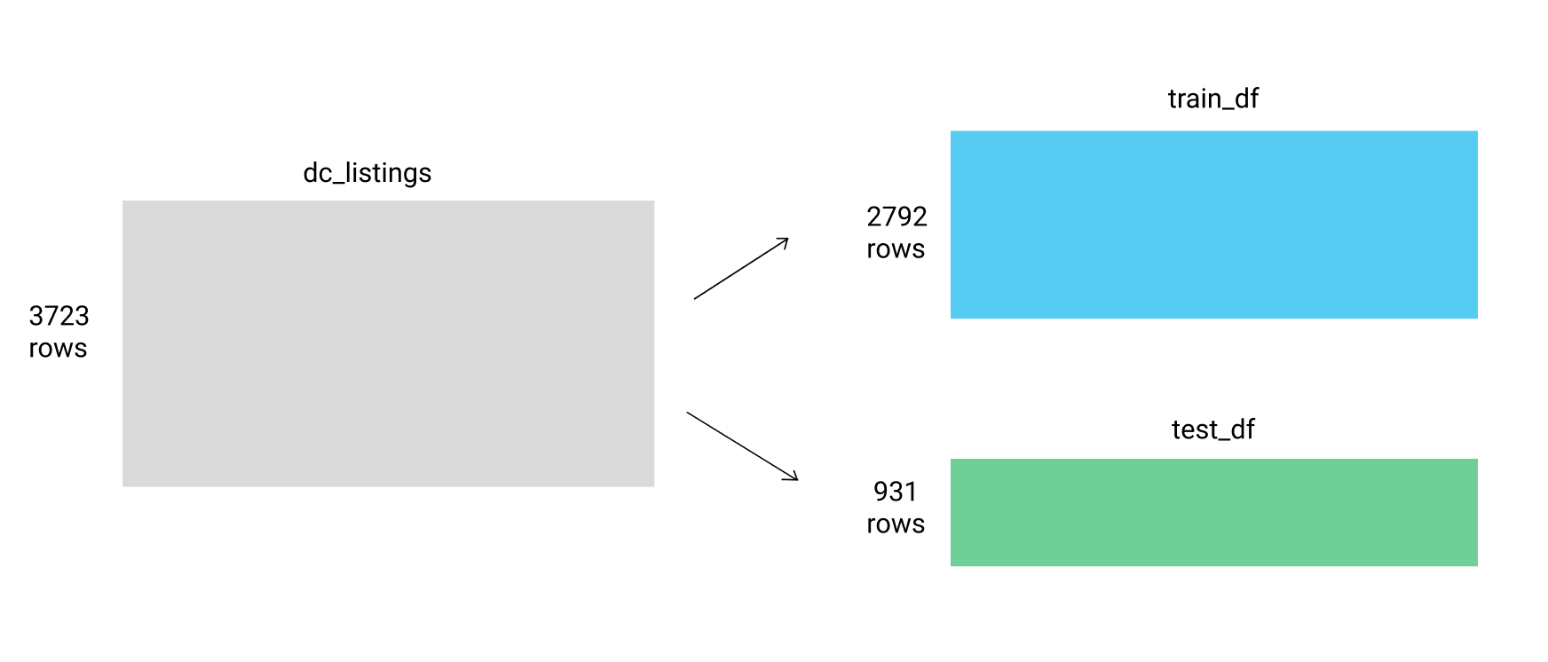
Splitting into train and test dataframes
We’ll also remove the column we added earlier when we created our first model.
dc_listings.drop('distance',axis=1)

train_df = dc_listings.copy().iloc[:2792]
test_df = dc_listings.copy().iloc[2792:]
To make things easier for ourselves while we look at metrics, we’ll combine the simple model we made earlier into a function. We won’t need to worry about randomizing the rows, since they’re still randomized from earlier.
def predict_price(new_listing_value,feature_column):
    temp_df = train_df
    temp_df['distance'] = np.abs(dc_listings[feature_column] - new_listing_value)
    temp_df = temp_df.sort_values('distance')
    knn_5 = temp_df.price.iloc[:5]
    predicted_price = knn_5.mean()
    return(predicted_price)
We can now use this function to predict values for our test dataset using the accommodates column.
test_df['predicted_price'] = test_df.accommodates.apply(predict_price,feature_column='accommodates')
Using RMSE to evaluate our model
For many prediction tasks, we want to penalize predicted values that are further away from the actual value much more than those that are closer to the actual value.
We can instead take the mean of the squared error values, which is called the root mean squared error (RMSE).
Here’s the formula for RMSE:
where n represents the number of rows in the test set.
This formular might look overwhelming at first, but all we’re doing is:
- Taking the difference between each predicted value and the actual value (or error),
- Squaring this difference (square),
- Taking the mean of all the squared differences (mean), and
- Taking the square root of that mean (root).
Hence, reading from bottom to top: root mean squared error.
Let’s calculate the RMSE value for the predictions we made on the test set.
test_df['squared_error'] = (test_df['predicted_price'] - test_df['price'])**(2)
mse = test_df['squared_error'].mean()
rmse = mse ** (1/2)
rmse
Our RMSE is about $213. One of the handy things about RMSE is that because we square and then take the square-root, the units for RMSE are the same as the value we are predicting, which makes it easy to understand the scale of our error.
Comparing different models
With an error metric that we can use to see the accuracy of our model, let’s create some predictions using different columns and look at how our error varies.
for feature in ['accommodates','bedrooms','bathrooms','number_of_reviews']:
    test_df['predicted_price'] = test_df.accommodates.apply(predict_price,feature_column=feature)

    test_df['squared_error'] = (test_df['predicted_price'] - test_df['price'])**(2)
    mse = test_df['squared_error'].mean()
    rmse = mse ** (1/2)
    print("RMSE for the {} column: {}".format(feature,rmse))
You can see that the best model of the four that we trained is the one using the accomodates column, however the error rates we’re getting are quite high relative to the range of prices of the listing in our data set.
So far, we’ve been training our model with only one feature, which is known as a univariate model. For more accuracy, we can use multiple features, which is known as a multivariate model.
We’re going to read in a cleaned version of this data set so that we can focus on evaluating the models. In our cleaned data set:
- All columns have been converted to numeric values, since we can’t calculate the Euclidean distance of a value with non-numeric characters.
- Non numeric columns have been removed for simplicity.
- Any listings with missing values have been removed.
- We have normalized the columns which will give us more accurate results.
If you’d like to read more about data cleaning and preparing data for machine learning, you can read the excellent post Preparing and Cleaning Data for Machine Learning.
Let’s read in this cleaned version, which is called dc_airbnb.normalized.csv, and preview the first few rows:
normalized_listings = pd.read_csv('dc_airbnb_normalized.csv')
print(normalized_listings.shape)
normalized_listings.head()
We’ll then randomize the rows and split it into a train and test dataset.
normalized_listings = normalized_listings.sample(frac=1,random_state=0)

norm_train_df = normalized_listings.copy().iloc[0:2792]
norm_test_df = normalized_listings.copy().iloc[2792:]
Calculating Euclidean distance with multiple features
Let’s remind ourselves what the original Euclidean distance equation looked like again:
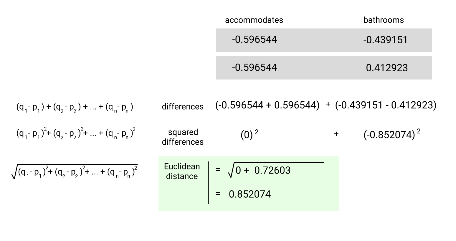
We’re going to start by building a model that uses the accommodates and bathrooms attributes. For this case, our Euclidean equation would look like:
To find the distance between two living spaces, we need to calculate the squared difference between both accommodates values, the squared difference between both bathrooms values, add them together, and then take the square root of the resulting sum. Here’s what the Euclidean distance between the first two rows in normalized_listings looks like:
So far, we’ve been calculating Euclidean distance ourselves by writing the logic for the equation ourselves. We can instead use the distance.euclidean() function from scipy.spatial, which takes in two vectors as the parameters and calculates the Euclidean distance between them. The euclidean() function expects:
- both of the vectors to be represented using a list-like object (Python list, NumPy array, or pandas Series)
- both of the vectors must be 1-dimensional and have the same number of elements
Let’s use the euclidean() function to calculate the Euclidean distance between the first and fifth rows in our dataset to practice.
from scipy.spatial import distance

first_listing = normalized_listings.iloc[0][['accommodates', 'bathrooms']]
fifth_listing = normalized_listings.iloc[20][['accommodates', 'bathrooms']]
first_fifth_distance = distance.euclidean(first_listing, fifth_listing)
first_fifth_distance
Creating a multivariate KNN model
We can extend our previous function to use two features and our whole data set. Instead of distance.euclidean(), we’re doing to use distance.cdist() since it allows us to pass multiple rows at once. The cdist() method can be used to calcuate distance using a variety of methods, but it defaults to Euclidean.
def predict_price_multivariate(new_listing_value,feature_columns):
    temp_df = norm_train_df
    temp_df['distance'] = distance.cdist(temp_df[feature_columns],[new_listing_value[feature_columns]])
    temp_df = temp_df.sort_values('distance')
    knn_5 = temp_df.price.iloc[:5]
    predicted_price = knn_5.mean()
    return(predicted_price)

cols = ['accommodates', 'bathrooms']
norm_test_df['predicted_price'] = norm_test_df[cols].apply(predict_price_multivariate,feature_columns=cols,axis=1)
norm_test_df['squared_error'] = (norm_test_df['predicted_price'] - norm_test_df['price'])**(2)
mse = norm_test_df['squared_error'].mean()
rmse = mse ** (1/2)
print(rmse)
You can see that our RMSE improved from 212 to 122 when using two features instead of just accommodates.
We’ve been writing functions from scratch to train the k-nearest neighbor models. While this is helpful to understand how the mechanics work, you can be more productive and iterate quicker by using a library that handles most of the implementation.
Scikit-learn is the most popular machine learning library in Python. Scikit-learn contains functions for all of the major machine learning algorithms and a simple, unified workflow. Both of these properties allow data scientists to be incredibly productive when training and testing different models on a new dataset.
The scikit-learn workflow consists of four main steps:
- Instantiate the specific machine learning model you want to use.
- Fit the model to the training data.
- Use the model to make predictions.
- Evaluate the accuracy of the predictions.
Each model in scikit-learn is implemented as a separate class and the first step is to identify the class we want to create an instance of. In our case, we want to use the KNeighborsRegressor class.
Any model that helps us predict numerical values, like listing price in our case, is known as a regression model. The other main class of machine learning models is called classification, where we’re trying to predict a label from a fixed set of labels (e.g. blood type or gender). The word regressor from the class name KNeighborsRegressor refers to the regression model class that we just discussed.
Scikit-learn uses a similar object-oriented style to Matplotlib and you need to instantiate an empty model first by calling the constructor.
from sklearn.neighbors import KNeighborsRegressor
knn = KNeighborsRegressor()
If you refer to the documentation, you’ll notice that by default:
n_neighbors: the number of neighbors, is set to5algorithm: for computing nearest neighbors, is set toautop: set to2, corresponding to Euclidean distance
Let’s set the algorithm parameter to brute and leave the n_neighbors value as 5, which matches the manual implementation we built.
from sklearn.neighbors import KNeighborsRegressor
knn = KNeighborsRegressor(algorithm='brute')
Now, we can fit the model to the data using the fit method. For all models, the fit method takes in two required parameters:
- matrix-like object, containing the feature columns we want to use from the training set.
- list-like object, containing correct target values.
Matrix-like object means that the method is flexible in the input and either a Dataframe or a NumPy 2D array of values is accepted. This means you can select the columns you want to use from the Dataframe and use that as the first parameter to the fit method.
If you recall from earlier, all of the following are acceptable list-like objects:
- NumPy array.
- Python list.
- pandas Series object (e.g. when selecting a column).
You can select the target column from the Dataframe and use that as the second parameter to the fit method:
knn.fit(train_features, train_target)
When the fit() method is called, scikit-learn stores the training data we specified within the KNearestNeighbors instance (knn). If you try passing in data containing missing values or non-numerical values into the fit method, scikit-learn will return an error. Scikit-learn contains many such features that help prevent us from making common mistakes.
Now that we specified the training data we want used to make predictions, we can use the predict method to make predictions on the test set. The predict method has only one required parameter:
- matrix-like object, containing the feature columns from the dataset we want to make predictions on
The number of feature columns you use during both training and testing need to match or scikit-learn will return an error:
predictions = knn.predict(test_features)
The predict() method returns a NumPy array containing the predicted price values for the test set. You now have everything you need to practice the entire scikit-learn workflow.
knn.fit(norm_train_df[cols], norm_train_df['price'])
two_features_predictions = knn.predict(norm_test_df[cols])
Calculating MSE using Scikit-Learn
Up until this point we have been calculating RMSE values manually, both using NumPy and SciPy functions to assist us. Alternatively, we can instead use the sklearn.metrics.mean_squared_error function(). Once you become familiar with the different machine learning concepts, unifying your workflow using scikit-learn helps save you a lot of time and helps you avoid mistakes.
The mean_squared_error() function takes in two inputs:
- A list-like object, representing the true values.
- A second list-like object, representing the predicted values using the model.
from sklearn.metrics import mean_squared_error

two_features_mse = mean_squared_error(norm_test_df['price'], two_features_predictions)
two_features_rmse = two_features_mse ** (1/2)
print(two_features_rmse)
Not only is this much simpler from a syntax perspective, but it also takes less time for the model to run as scikit-learn has been heavily optimized for speed.
You’ll notice that our RMSE is a little different from our manually implemented algorithm — this is likely due to both differences in the randomization and slight differences in implementation between our ‘manual’ KNN algorithm and the scikit-learn version.
Using more features
One of the best things about scikit-learn is that it allows us to iterate quicker.
Let’s see this in action, by creating a model which uses four features instead of two and see if that improves our results.
knn = KNeighborsRegressor(algorithm='brute')

cols = ['accommodates','bedrooms','bathrooms','beds']

knn.fit(norm_train_df[cols], norm_train_df['price'])
four_features_predictions = knn.predict(norm_test_df[cols])
four_features_mse = mean_squared_error(norm_test_df['price'], four_features_predictions)
four_features_rmse = four_features_mse ** (1/2)
four_features_rmse
In this case, our error went down slightly, but it may not always do so as you add features.
This is an important thing to be aware of – more features does not necessarily make an accurate model, since adding a feature that is not an accurate predictor of your target variable adds ‘noise’ to your model.
Summary
Let’s take a look at what we’ve learned:
- We learned what machine learning is.
- We learned about the k-nearest neighbors algorithm, and built a univariate model (only one feature) from scratch and used it to make predictions.
- We learned that RMSE can be used to calculate the error of our models, which we can then use to iterate and try and improve our predictions.
- We then created a multivariate (more than one feature) model from scratch and used that to make predictions.
- Finally, we learned about the scikit-learn library, and used the
KNeighborsRegressorclass to make predictions.
Next Steps
If you’d like to learn more, this tutorial is based on our Dataquest Machine Learning Fundamentals course, which is part of our Data Science Learning Path. The course goes into a lot more detail and extends on the model built in this post, while allowing you to follow along writing code to learn by doing.
If you’d like to continue working on this model on your own, here are a few things you can to do improve accuracy: