When working with classification and/or regression techniques, its always good to have the ability to ‘explain’ what your model is doing. Using Local Interpretable Model-agnostic Explanations (LIME), you now have the ability to quickly provide visual explanations of your model(s).
Its quite easy to throw numbers or content into an algorithm and get a result that looks good. We can test for accuracy and feel confident that the classifier and/or model is ‘good’…but can we describe what the model is actually doing to other users? A good data scientist spends some of their time making sure they have reasonable explanations for what the model is doing and why the results are what they are.
There’s always been a focus on ‘trust’ in any type of modeling methodology but with machine learning and deep learning, many people feel like the black-box approach taken with these methods isn’t as trustworthy as other methods. This topic was addressed in a paper titled Why Should I Trust You?”: Explaining the Predictions of Any Classifier, which proposes the concept of Local Interpretable Model-agnostic Explanations (LIME). According to the paper, LIME is ‘an algorithm that can explain the predictions of any classifier or regressor in a faithful way, by approximating it locally with an interpretable model.’
I’ve used the LIME approach a few times in recent projects and really like the idea. It breaks down the modeling / classification techniques and output into a form that can be easily described to non-technical people. That said, LIME isn’t a replacement for doing your job as a data scientist, but it is another tool to add to your toolbox.
To implement LIME in python, I use this LIME library written / released by one of the authors the above paper.
I thought it might be good to provide a quick run-through of how to use this library. For this post, I’m going to mimic “Using lime for regression” notebook the authors provide, but I’m going to provide a little more explanation.
The full notebook is available in my repo here.
Getting started with Local Interpretable Model-agnostic Explanations (LIME)
Before you get started, you’ll need to install Lime.
pip install lime
Next, let’s import our required libraries.
from sklearn.datasets import load_boston
import sklearn.ensemble
import numpy as np
from sklearn.model_selection import train_test_split
import lime
import lime.lime_tabular
Let’s load the sklearn dataset called ‘boston’. This data is a dataset that contains house prices that is often used for machine learning regression examples.
boston = load_boston()
Before we do much else, let’s take a look at the description of the dataset to get familiar with it. You can do this by running the following command:
print boston['DESCR']
The output is:
Boston House Prices dataset
===========================

Notes
------
Data Set Characteristics:

    :Number of Instances: 506

    :Number of Attributes: 13 numeric/categorical predictive

    :Median Value (attribute 14) is usually the target

    :Attribute Information (in order):
        - CRIM     per capita crime rate by town
        - ZN       proportion of residential land zoned for lots over 25,000 sq.ft.
        - INDUS    proportion of non-retail business acres per town
        - CHAS     Charles River dummy variable (= 1 if tract bounds river; 0 otherwise)
        - NOX      nitric oxides concentration (parts per 10 million)
        - RM       average number of rooms per dwelling
        - AGE      proportion of owner-occupied units built prior to 1940
        - DIS      weighted distances to five Boston employment centres
        - RAD      index of accessibility to radial highways
        - TAX      full-value property-tax rate per $10,000
        - PTRATIO  pupil-teacher ratio by town
        - B        1000(Bk - 0.63)^2 where Bk is the proportion of blacks by town
        - LSTAT    % lower status of the population
        - MEDV     Median value of owner-occupied homes in $1000's

    :Missing Attribute Values: None

    :Creator: Harrison, D. and Rubinfeld, D.L.

This is a copy of UCI ML housing dataset.
http://archive.ics.uci.edu/ml/datasets/Housing


This dataset was taken from the StatLib library which is maintained at Carnegie Mellon University.

The Boston house-price data of Harrison, D. and Rubinfeld, D.L. 'Hedonic
prices and the demand for clean air', J. Environ. Economics & Management,
vol.5, 81-102, 1978.   Used in Belsley, Kuh & Welsch, 'Regression diagnostics
...', Wiley, 1980.   N.B. Various transformations are used in the table on
pages 244-261 of the latter.

The Boston house-price data has been used in many machine learning papers that address regression
problems.

**References**

   - Belsley, Kuh & Welsch, 'Regression diagnostics: Identifying Influential Data and Sources of Collinearity', Wiley, 1980. 244-261.
   - Quinlan,R. (1993). Combining Instance-Based and Model-Based Learning. In Proceedings on the Tenth International
         Conference of Machine Learning, 236-243, University of Massachusetts, Amherst. Morgan Kaufmann.
   - many more! (see http://archive.ics.uci.edu/ml/datasets/Housing)
Now that we have our data loaded, we want to build a regression model to forecast boston housing prices. We’ll use random forest for this to follow the example by the authors.
First, we’ll set up the RF Model and then create our training and test data using the train_test_split module from sklearn. Then, we’ll fit the data.
rf = sklearn.ensemble.RandomForestRegressor(n_estimators=1000)
train, test, labels_train, labels_test = train_test_split(boston.data, boston.target, train_size=0.80)
rf.fit(train, labels_train)
Now that we have a Random Forest Regressor trained, we can check some of the accuracy measures.
print('Random Forest MSError', np.mean((rf.predict(test) - labels_test) ** 2))
Tbe MSError is: 10.45. Now, let’s look at the MSError when predicting the mean.
print('MSError when predicting the mean', np.mean((labels_train.mean() - labels_test) ** 2))
From this, we get 80.09.
Without really knowing the dataset, its hard to say whether they are good or bad. Since we are really most interested in looking at the LIME approach, we’ll move along and assume these are decent errors.
To implement LIME, we need to get the categorical features from our data and then build an ‘explainer’. This is done with the following commands:
categorical_features = np.argwhere(
    np.array([len(set(boston.data[:,x]))
    for x in range(boston.data.shape[1])]) <= 10).flatten()
and the explainer:
explainer = lime.lime_tabular.LimeTabularExplainer(train,
                                                   feature_names=boston.feature_names,
                                                   class_names=['price'],
                                                   categorical_features=categorical_features,
                                                   verbose=True, mode='regression')
Now, we can grab one of our test values and check out our prediction(s). Here, we’ll grab the 100th test value and check the prediction and see what the explainer has to say about it.
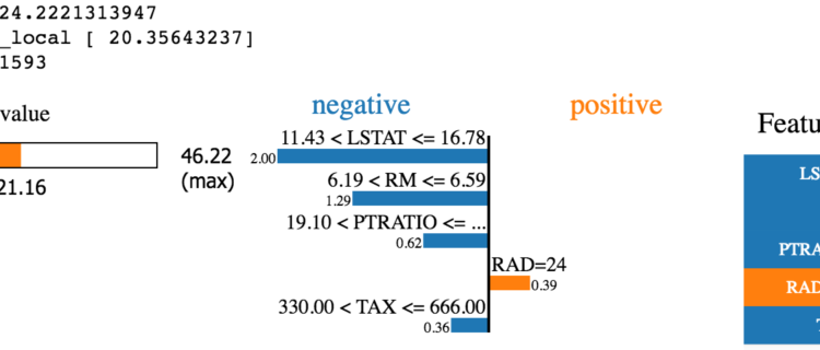
i = 100

exp = explainer.explain_instance(test[i], rf.predict, num_features=5)
exp.show_in_notebook(show_table=True)
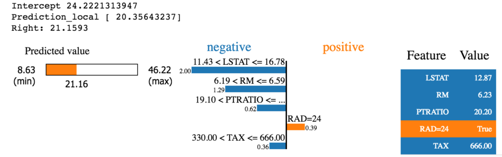
So…what does this tell us?
It tells us that the 100th test value’s prediction is 21.16 with the “RAD=24” value providing the most positive valuation and the other features providing negative valuation in the prediction.
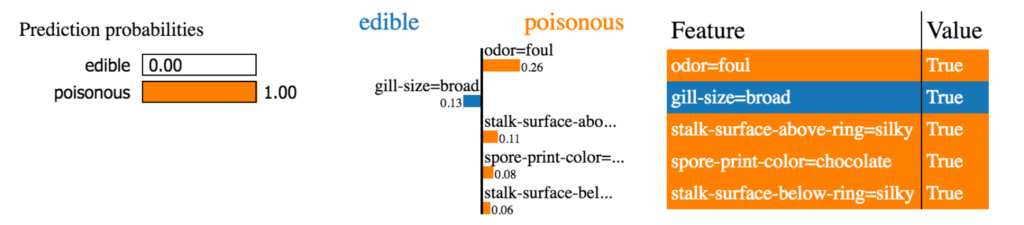
For regression, this isn’t quite as interesting (although it is useful). The LIME approach shows much more benefit (at least to me) when performing classification.
As an example, if you are trying to classify plans as edible or poisonous, LIME’s explanation is much more useful. Here’s an example from the authors.
Take a look at LIME when you have some time. Its a good library to add to your toolkit, especially if you are doing a lot of classification work. It makes it much easier to ‘explain’ what the model is doing.
The post Local Interpretable Model-agnostic Explanations – LIME in Python appeared first on Python Data.