Forecasting Time-Series data with Prophet – Part 1

This is part 1 of a series where I look at using Prophet for Time-Series forecasting in Python

A lot of what I do in my data analytics work is understanding time series data, modeling that data and trying to forecast what might come next in that data. Over the years I’ve used many different approaches, library and modeling techniques for modeling and forecasting with some success…and a lot of failure.

Recently, I’ve been looking for a simpler approach for my initial modeling and think I’ve found a very nice library in Facebook’s Prophet (available for both python and R). While this particular library isn’t terribly robust, it is quick and gives some very good results for that initial pass at modeling / forecasting time series data. An added bonus with Prophet for those that like to understand the theory behind things is this white paper with a very good description of the math / statistical approach behind Prophet.

If you are interested in learning more about time-series forecasting, check out the books / websites below.

Installing Prophet

To get started with Prophet, you’ll first need to install it (of course).

Installation instructions can be found here, but it should be as easy as doing the following (if you have an existing system that has the proper compilers installed):

pip install fbprophet

For those running conda, you can install prophet via conda-forge using the following command:

conda install -c conda-forge fbprophet

Note: Prophet requres pystan, so you may need to also do the following (although in my case, it was installed as a requirement of fbprophet):

pip install pystan

Pystan documentation can be found here.

Getting started

Using Prophet is extremely straightforward. You import it, load some data into a pandas dataframe, set the data up into the proper format and then start modeling / forecasting.

First, import the module (plus some other modules that we’ll need):

from fbprophet import Prophet
import numpy as np
import pandas as pd

Now, let’s load up some data. For this example, I’m going to be using the retail sales example csv file find on github.

sales_df = pd.read_csv('../examples/retail_sales.csv')

Now, we have a pandas dataframe with our data that looks something like this:

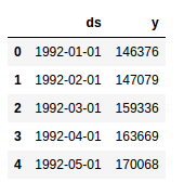
Note the format of the dataframe. This is the format that Prophet expects to see. There needs to be a ‘ds’ column that contains the datetime field and and a ‘y’ column that contains the value we are wanting to model/forecast.

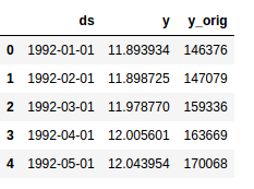
Before we can do any analysis with this data, we need to log transform the ‘y’ variable to a try to convert non-stationary data to stationary. This also converts trends to more linear trends (see this website for more info). This isn’t always a perfect way to handle time-series data, but it works often enough that it can be tried initially without much worry.

To log-tranform the data, we can use np.log() on the ‘y’ column like this:

sales_df['y_orig'] = sales_df['y'] # to save a copy of the original data..you'll see why shortly. 
# log-transform y
sales_df['y'] = np.log(sales_df['y'])

Your dataframe should now look like the following:

Its time to start the modeling. You can do this easily with the following command:

model = Prophet() #instantiate Prophet
model.fit(sales_df); #fit the model with your dataframe

If you are running with monthly data, you’ll most likely see the following message after you run the above commands:

Disabling weekly seasonality. Run prophet with weekly_seasonality=True to override this.

You can ignore this message since we are running monthly data.

Now its time to start forecasting. With Prophet, you start by building some future time data with the following command:

future_data = model.make_future_dataframe(periods=6, freq = 'm')

In this line of code, we are creating a pandas dataframe with 6 (periods = 6) future data points with a monthly frequency (freq = ‘m’). If you’re working with daily data, you wouldn’t want include freq=’m’.

Now we forecast using the ‘predict’ command:

<span class="n">forecast_data</span> <span class="o">=</span> <span class="n">m</span><span class="o">.</span><span class="n">predict</span><span class="p">(</span><span class="n">future_data</span><span class="p">)</span>

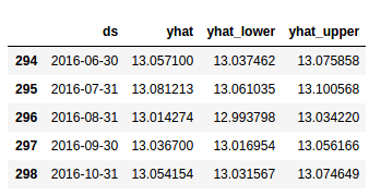
If you take a quick look at the data using .head() or .tail(), you’ll notice there are a lot of columns in the forecast_data dataframe. The important ones (for now) are ‘ds’ (datetime), ‘yhat’ (forecast), ‘yhat_lower’ and ‘yhat_upper’ (uncertainty levels).

You can view only these columns in a .tail() by running the following command.

forecast_data[['ds', 'yhat', 'yhat_lower', 'yhat_upper']].tail()

Your dataframe should look like:

Let’s take a look at a graph of this data to get an understanding of how well our model is working.

itmodel.plot(forecast_data)

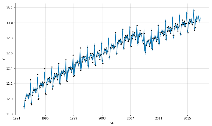
That looks pretty good. Now, let’s take a look at the seasonality and trend components of our /data/model/forecast.

model.plot_components(forecast_data)

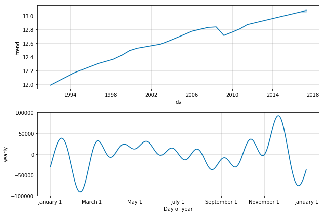
Since we are working with monthly data, Prophet will plot the trend and the yearly seasonality but if you were working with daily data, you would also see a weekly seasonality plot included.

From the trend and seasonality, we can see that the trend is a playing a large part in the underlying time series and seasonality comes into play more toward the beginning and the end of the year.

So far so good. With the above info, we’ve been able to quickly model and forecast some data to get a feel for what might be coming our way in the future from this particular data set.

Before we go on to tweaking this model (which I’ll talk about in my next post), I wanted to share a little tip for getting your forecast plot to display your ‘original’ data so you can see the forecast in ‘context’ and in the original scale rather than the log-transformed data. You can do this by using np.exp() to get our original data back.

forecast_data_orig = forecast_data # make sure we save the original forecast data
forecast_data_orig['yhat'] = np.exp(forecast_data_orig['yhat'])
forecast_data_orig['yhat_lower'] = np.exp(forecast_data_orig['yhat_lower'])
forecast_data_orig['yhat_upper'] = np.exp(forecast_data_orig['yhat_upper'])

Let’s take a look at the forecast with the original data:

model.plot(forecast_data_orig)

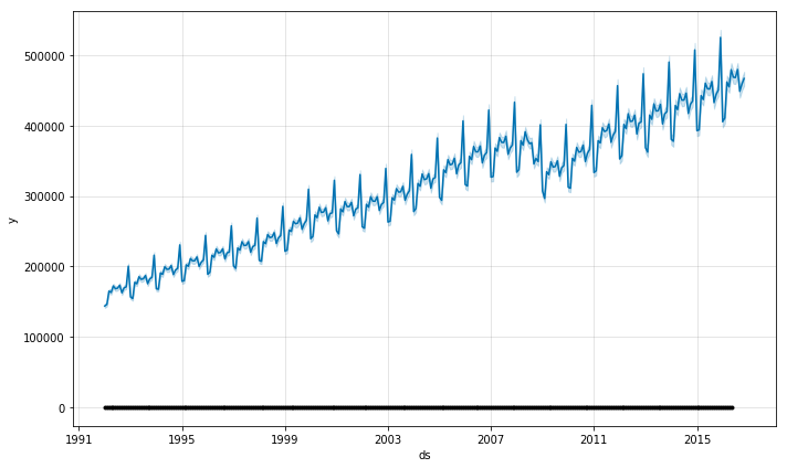
Something looks wrong (and it is)!

Our original data is drawn on the forecast but the black dots (the dark line at the bottom of the chart) is our log-transform original ‘y’ data. For this to make any sense, we need to get our original ‘y’ data points plotted on this chart. To do this, we just need to rename our ‘y_orig’ column in the sales_df dataframe to ‘y’ to have the right data plotted. Be careful here…you want to make sure you don’t continue analyzing data with the non-log-transformed data.

sales_df['y_log']=sales_df['y'] #copy the log-transformed data to another column
sales_df['y']=sales_df['y_orig'] #copy the original data to 'y'

And…plot it.

model.plot(forecast_data_orig)

There we go…a forecast for retail sales 6 months into the future (you have to look closely at the very far right-hand side for the forecast). It looks like the next six months will see sales between 450K and 475K.

Check back soon for my next post on using Prophet for forecasting time-series data where I talk about how to tweak the models that come out of prophet.

The post Forecasting Time-Series data with Prophet – Part 1 appeared first on Python Data.