Forecasting Time-Series data with Prophet – Part 2

In Forecasting Time-Series data with Prophet – Part 1, I introduced Facebook’s Prophet library for time-series forecasting.   In this article, I wanted to take some time to share how I work with the data after the forecasts. Specifically, I wanted to share some tips on how I visualize the Prophet forecasts using matplotlib rather than relying on the default prophet charts (which I’m not a fan of).

Just like part 1, I’m going to be using this retail sales example csv file find on github.

For this work, we’ll need to import matplotlib and set up some basic parameters to be format our plots in a nice way (unlike the hideous default matplotlib format).

from fbprophet import Prophet
import numpy as np
import pandas as pd
import matplotlib.pyplot as plt

%matplotlib inline #only needed for jupyter
plt.rcParams['figure.figsize']=(20,10)
plt.style.use('ggplot')

With this chunk of code, we import fbprophet, numpy, pandas and matplotlib. Additionally, since I’m working in jupyter notebook, I want to add the %matplotlib inline instruction to view the charts that are created during the session. Lastly, I set my figuresize and sytle to use the ‘ggplot’ style.

Since I’ve already described the analysis phase with Prophet, I’m not going to provide commentary on it here. You can jump back to Part 1 for a walk-through.

sales_df = pd.read_csv('examples/retail_sales.csv')

sales_df['y_orig']=sales_df.y # We want to save the original data for later use
sales_df['y'] = np.log(sales_df['y']) #take the log of the data to remove trends, etc

model = Prophet()
model.fit(sales_df);

#create 12 months of future data
future_data = model.make_future_dataframe(periods=12, freq = 'm')

#forecast the data for future data
forecast_data = model.predict(future_data)

At this point, your data should look like this:

 

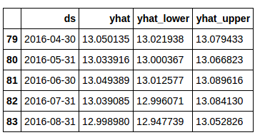
Now, let’s plot the output using Prophet’s built-in plotting capabilities.

model.plot(forecast_data)

 

 

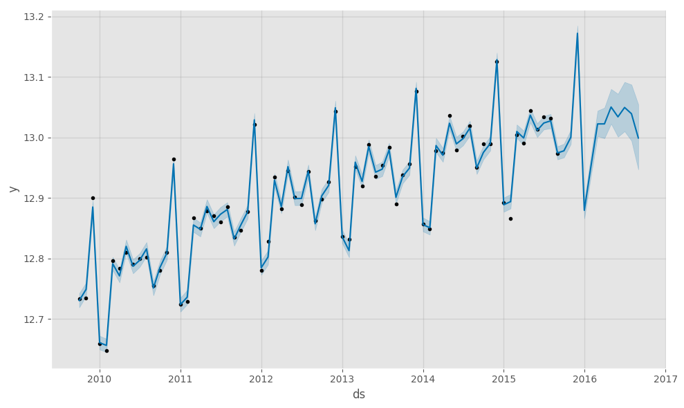
While this is a nice chart, it is kind of ‘busy’ for me.  Additionally, I like to view my forecasts with original data first and forecasts appended to the end (this ‘might’ make sense in a minute).

First, we need to get our data combined and indexed appropriately to start plotting. We are only interested (at least for the purposes of this article) in the ‘yhat’, ‘yhat_lower’ and ‘yhat_upper’ columns from the Prophet forecasted dataset.  Note: There are much more pythonic ways to these steps, but I’m breaking them out for each of understanding.

sales_df.set_index('ds', inplace=True)
forecast_data.set_index('ds', inplace=True)
viz_df = sales_df.join(forecast_data[['yhat', 'yhat_lower','yhat_upper']], how = 'outer')
del viz_df['y']
del viz_df['index']

You don’t need to delete the ‘y’and ‘index’ columns, but it makes for a cleaner dataframe.

If you ‘tail’ your dataframe, your data should look something like this:

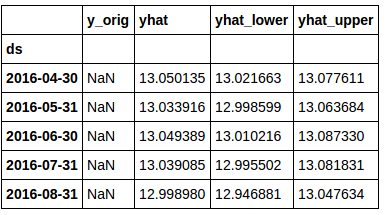
You’ll notice that the ‘y_orig’ column is full of “NaN” here. This is due to the fact that there is no original data for the ‘future date’ rows.

Now, let’s take a look at how to visualize this data a bit better than the Prophet library does by default.

First, we need to get the last date in the original sales data. This will be used to split the data for plotting.

sales_df.index = pd.to_datetime(sales_df.index)
last_date = sales_df.index[-1]

To plot our forecasted data, we’ll set up a function (for re-usability of course). This function imports a couple of extra libraries for subtracting dates (timedelta) and then sets up the function.

from datetime import date,timedelta

def plot_data(func_df, end_date):
    end_date = end_date - timedelta(weeks=4) # find the 2nd to last row in the data. We don't take the last row because we want the charted lines to connect
    mask = (func_df.index > end_date) # set up a mask to pull out the predicted rows of data.
    predict_df = func_df.loc[mask] # using the mask, we create a new dataframe with just the predicted data.
   
# Now...plot everything
    fig, ax1 = plt.subplots()
    ax1.plot(sales_df.y_orig)
    ax1.plot((np.exp(predict_df.yhat)), color='black', linestyle=':')
    ax1.fill_between(predict_df.index, np.exp(predict_df['yhat_upper']), np.exp(predict_df['yhat_lower']), alpha=0.5, color='darkgray')
    ax1.set_title('Sales (Orange) vs Sales Forecast (Black)')
    ax1.set_ylabel('Dollar Sales')
    ax1.set_xlabel('Date')
  
# change the legend text
    L=ax1.legend() #get the legend
    L.get_texts()[0].set_text('Actual Sales') #change the legend text for 1st plot
    L.get_texts()[1].set_text('Forecasted Sales') #change the legend text for 2nd plot

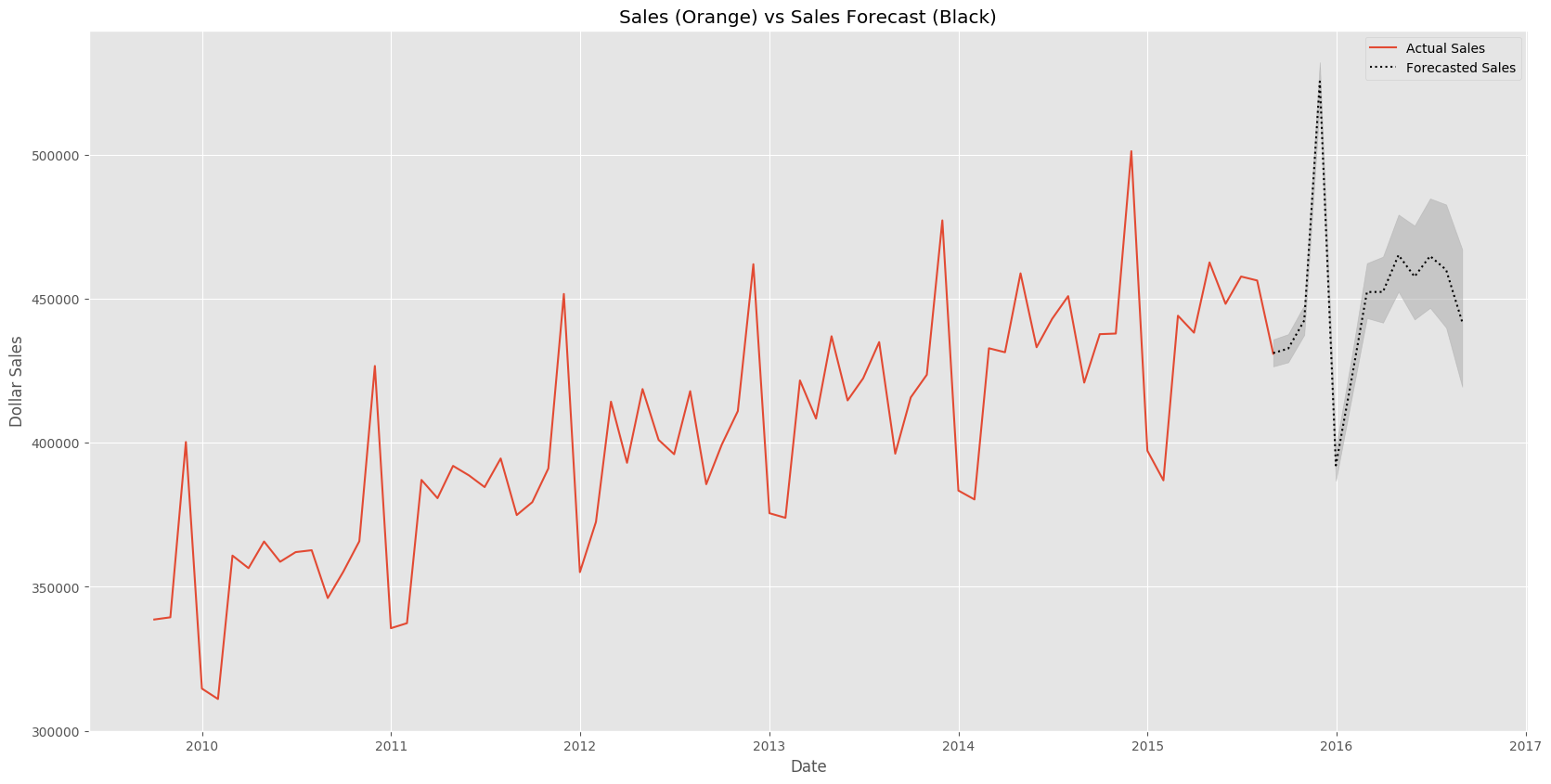
This function does a few simple things. It finds the 2nd to last row of original data and then creates a new set of data (predict_df) with only the ‘future data’ included. It then creates a plot with confidence bands along the predicted data.

The ploit should look something like this:

---

Hopefully you’ve found some useful information here. Check back soon for Part 3 of my Forecasting Time-Series data with Prophet.

The post Forecasting Time-Series data with Prophet – Part 2 appeared first on Python Data.